Concept 5: Kullback–Leibler Divergence
We are familiar with the entropy and the cross-entropy concepts, so we are gonna discuss about details of KL divergence here.
Definition of KL divergence
The KL divergence tells us how well the probability distribution Q approximates the probability distribution P by calculating the cross-entropy minus the entropy.

The cross-entropy and the entropy formulas are as below:


So the KL divergence can also be expressed in the expectation form as follows:
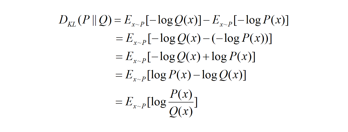
The expectation formula can be expressed in the discrete summation form or in the continuous integration form:

So, what does the KL divergence measure? It measures the similarity (or dissimilarity) between two probability distributions.
If so, is the KL divergence a distance measure?
To answer this question, let’s see a few more characteristics of the KL divergence.
The KL divergence is non-negative
The KL divergence is non-negative. An intuitive proof is that:
-
if P=Q, the KL divergence is zero as:

-
if P≠Q, the KL divergence is positive because the entropy is the minimum average lossless encoding size.
So, the KL divergence is a non-negative value that indicates how close two probability distributions are.
It does sound like a distance measure, doesn’t it? But it is not.
The KL divergence is asymmetric
The KL divergence is not symmetric:

It can be deduced from the fact that the cross-entropy itself is asymmetric. The cross-entropy H(P, Q) uses the probability distribution P to calculate the expectation. The cross-entropy H(Q, P) uses the probability distribution Q to calculate the expectation.
So, the KL divergence cannot be a distance measure as a distance measure should be symmetric.
This asymmetric nature of the KL divergence is a crucial aspect. Let’s look at two examples to understand it intuitively.
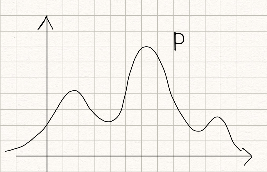
Suppose we have a probability distribution P which looks like below:
Now, we want to approximate it with a normal distribution Q as below:
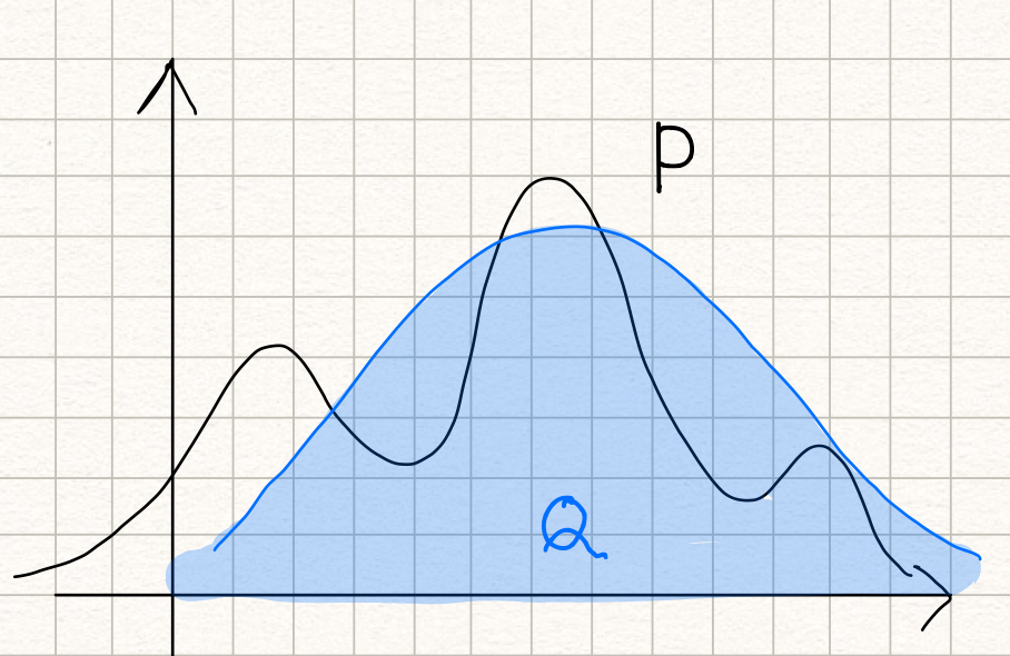
The KL divergence is the measure of inefficiency in using the probability distribution Q to approximate the true probability distribution P.

If we swap P and Q, it means that we use the probability distribution P to approximate the normal distribution Q, and it’d look like below:
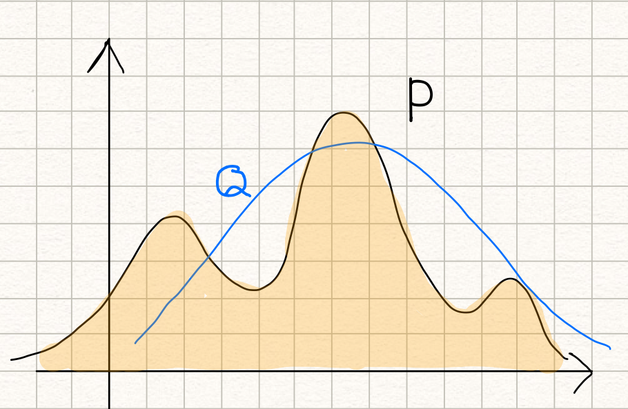

Both cases measure the similarity between P and Q, but the result could be entirely different, and they are both useful.
Modeling a true distribution
By approximating a probability distribution with a well-known distribution like the normal distribution, binomial distribution, etc., we are modeling the true distribution with a known one.
This is when we are using the below formula:
Calculating the KL divergence, we can find the model (the distribution and the parameters) that fits the true distribution well.
Variational Auto-encoder
An example of using the below formula is the variational auto-encoder.