Paper 1: Trust Region Policy Optimization (TRPO)
Abstract
-
A method for optimizing control policies, with guaranteed monotonic improvement
-
Making several approximations to the theoretically-justified scheme
-
Effective for optimizing large nonlinear policies, such as neural networks
-
Robust performance on a wide variety of tasks
-
Despite its approximations that deviate from the theory, TRPO tends to give monotonic improvement
1 Introduction
Most algorithms for policy optimization can be classified into three categories: policy iteration methods, which alternate between estimating the value function under the current policy and improving the policy; policy gradient methods, which use an estimator of the gradient of the expected cost obtained from sample trajectories (have a close connection to policy iteration); derivative-free optimization methods.
In this article, we first prove that minimizing a certain surrogate loss function guarantees policy improvement with non-trivial step sizes. Then we make a series of approximations to the theoretically-justified algorithm, yielding a practical algorithm.
We describe two variants of this algorithm: first, the single-path method, which can be applied in the model-free setting; second, the vine-method, which requires the system to be stored to particle states, which is typically only possible in simulation.
2 Preliminaries
Let η(π) denote its expected discounted rewards:

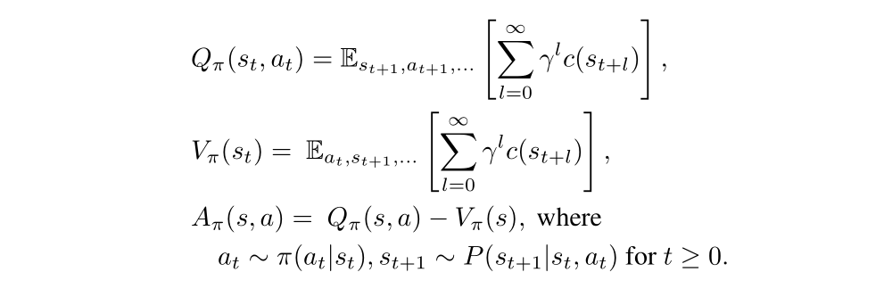
Standard definitions of the state-action value function Qπ, the value function Vπ, and the advantage function Aπ:
The following useful identity expresses the expected cost of another policy π bar, in terms of the advantage over π:

We want the second term on the right-hand side of Equation(1) to be positive to update the policy, but the equation now can’t give us much information, so we rearrange the Equation(1) to sum over states instead of time steps.
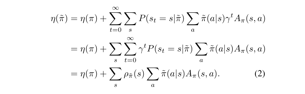
In Equation(2), we let ρπ be the (unnormalized) discounted visitation frequencies:

The Equation(2) implies that any policy update from π to π bar that has a nonnegative expected advantage at every state s. However, in the approximate setting, due to estimation and approximation error, there’ll be some states s for which the expected advantage is negative. The complex dependency of ρπ bar(s) on π bar makes Equation(2) difficult to optimize directly. Instead, we introduce the following local approximation to η:

The Lπ uses the visitation sequence ρπ rather ρπ bar, ignoring changes in state visitation density due to changes in policy. However, if we have a parameterized policy πθ, where πθ(a|s) is a differentiable function of the parameter vector θ, then Lπ matches η to first order. That is, for any parameter value θ0,

Equation(4) implies that a sufficiently small step from πθ0 to π bar that improves Lπθold will also improve η, but doesn’t give us any guidance on how big of a step to take.

To address this, Kakade & Langford (2002) proposed a policy updating scheme called conservative (保守的)policy iteration, for which we could provide explicit lower bounds on the improvement of η.
The new policy πnew was defined to be the following mixture:

Kakade and Langford derived the following lower bound:

However, that so far this bound only applies to mixture policies generated by Equation (5). This policy class is unwieldy and restrictive in practice, and it is desirable for a practical policy update scheme to be applicable to all general stochastic policy classes.
3 Monotonic Improvement Guarantee for General Stochastic Policies
Equation(6), which applies to conservative policy iteration, implies that a policy update that improves the right-hand side is guaranteed to improve the true performance η. Our principal theoretical result is that the policy improvement bound in Equation (6) can be extended to general stochastic policies, rather than just mixture polices, by replacing α with a distance measure between π and π bar. Since mixture policies are rarely used in practice, this result is crucial for extending the improvement guarantee to practical problems. The particular distance measure we use is the total variation divergence, which is defined by:

for discrete probability distribution p,q. Then we define:

What we are going to do is to introduce the proof of policy improvement bound. We need some techniques. Our proof relies on the notion of coupling, where we jointly define the policies π and π’ so that they choose the same action with high probability 1- α. Surrogate loss Lπ(π bar) accounts for the advantage of π bar the first time that it disagrees with π, but not subsequent disagreements. Hence, the error in Lπ is due to two or more disagreements between π and π bar, we get an O(α2) correction term, where α is the probability of disagreement.
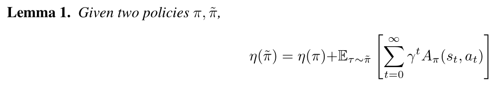
We start out with the lemma that shows the difference in policy performance η(π bar) - η(π), can be decomposed as a sum of per-timestep advantages.
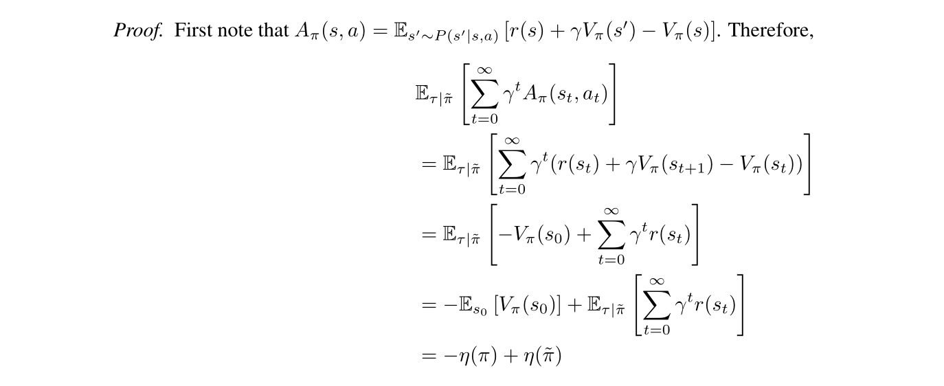
And its proof is as belows:
We define A bar(s) to be the expected advantage of π bar over π at state s:

Then the Lemma 1 can be written as follows:

The Lπ(π bar) can be written as:

This is our first approximation!
To bound the difference between η(π bar) and Lπ(π bar), we’ll bound the difference arising from each timestep. To do this, we first need to introduce a measure of how much π and π bar agree. Specifically, we’ll couple the policies, so that they define a joint distribution over pairs of actions.
Definition: (π, π bar) is an α-coupled policy pair if it defines a joint distribution (a, a bar)|s, such that P(a is not equal to a bar|s) is less than or equal to α for all s. π and π bar will denote marginal distributions of a and a bar, respectively.
Computationally, α-coupling means that if we randomly choose a seed for our random number generator, and then we sample from each of π and π bar after setting that seed, the results will agree for at least fraction 1- α of seeds. From the definition above, we can get Lemma 2.
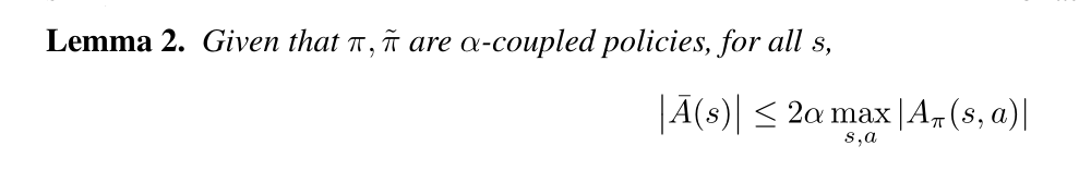
And its proof is as belows:
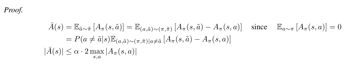
We can also get the Lemma 3:
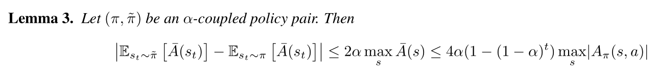
Since we have pairs of trajectories, to prove the Lemma 3, we will consider the advantage of π bar over π at timestep t, and decompose this expectation based on whether π agrees with π bar at all timesteps i<t.
Let nt denote the number of times that ai is not equal to ai bar for i<t, i.e., the number of times that π and π bar disagree before timestep t.

The expectation decomposes similarly for actions are sampled using π:

Note that the nt = 0 terms are equal because nt = 0 indicates that π and π bar agreed on all timesteps less than t:

Subtracting the equations above, we can get:

By definition of α, P(π, π bar agree at timestep i) is more than or equal to 1-α, we can get:

Then we can get:

According to Lemma 2, it’s easy for us to get:
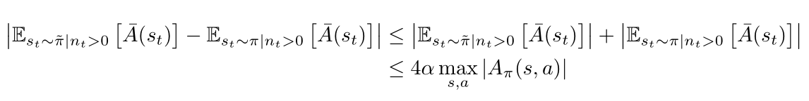
Through plugging into equation, we can get:

The preceding Lemma bounds the difference in expected advantage at each timestep t. We can sum over time to bound the difference between η(π bar) and Lπ(π bar). We define:

Then we can get:
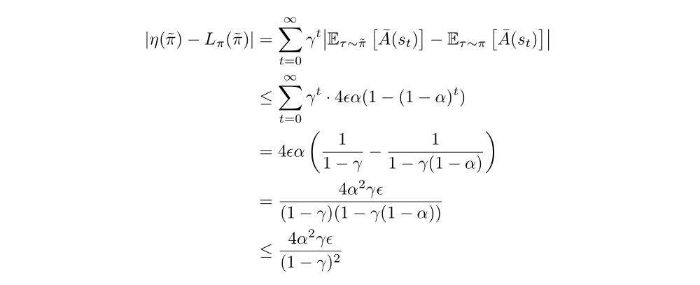
Last, to replace α by the total variation divergence, we need to use the correspondence between TV divergence and coupled random variables. The fact is that the random variables from two distributions with total variation divergence less than α can be coupled, so that they are equal with probability 1 − α.

Based on the above derivation, we can get Theorem 1:
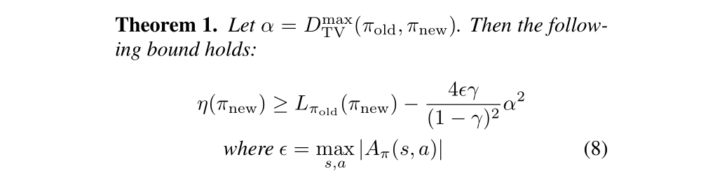
Next, we note the following relationship between the total variation divergence and the KL divergence:

Let

The following bound then follows directly from Theorem 1:

It's a very important inequation!
Based on the policy improvement bound in Equation(9), we get the Algorithm 1, which describes an approximate policy iteration scheme.
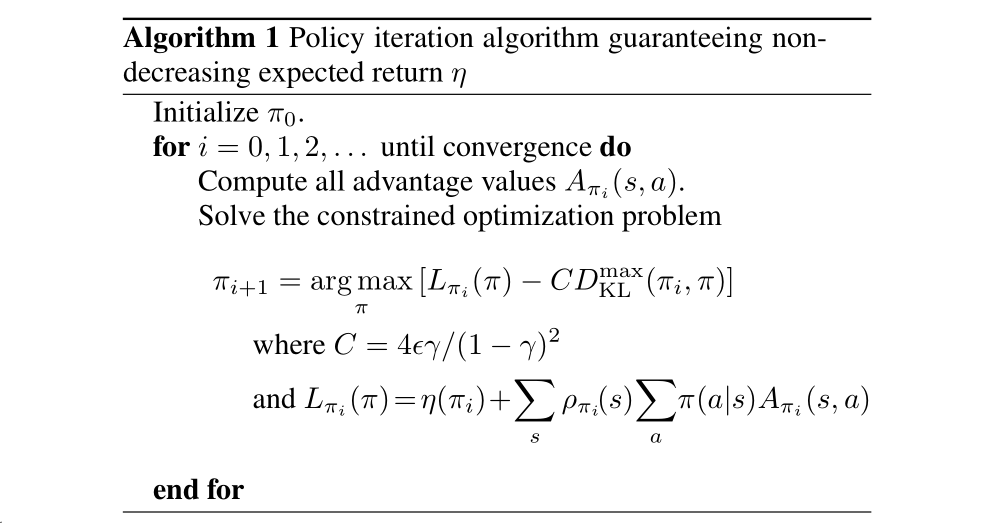
It follows from Equation(9) that Algorithm 1 is guaranteed to generate a monotonically improving sequence of policies:

To see this, let Mi(π) denote the right-hand side of Equation(9).

Then

Thus, by maximizing Mi in each iteration, we guarantee that the true objective η is non-decreasing. For now, we assume exact evaluation of the advantage values Aπ.
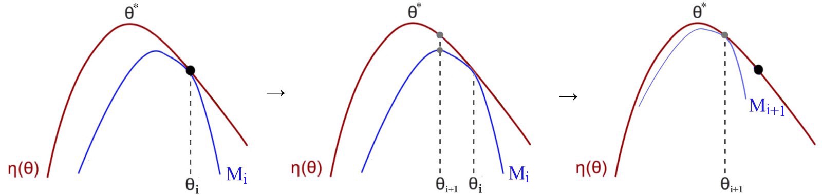
The Algorithm 1 is a type of minorization-maximization (MM) algorithm, which is a class of methods that also includes expectation maximization.
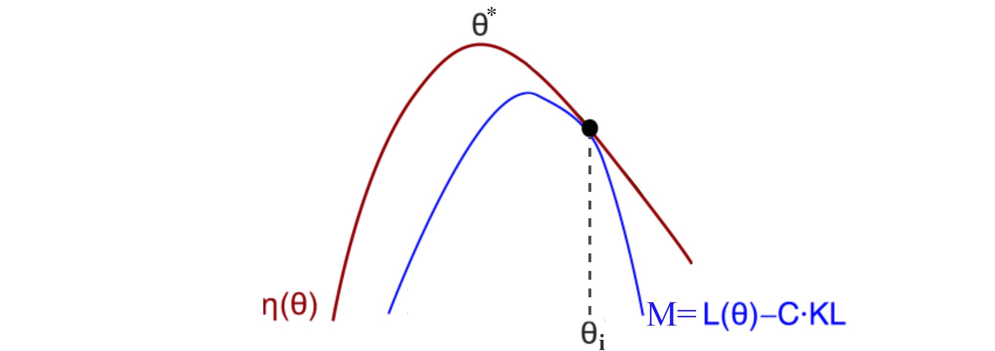
MM is an iterative method. For each iteration, we find a surrogate function M (the blue curve) that is: (1) a lower bound function for η, (2) approximate η at the current policy, and (2) easy to optimize (we will approximate the surrogate function as a quadratic equation).
In each iteration, we find the optimal point for M and use that as the current policy.
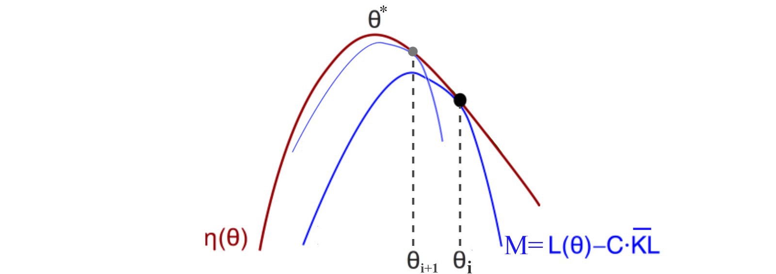
Then, we re-evaluate a lower bound at the new policy and repeat the iteration. As we continue the process, the policy keeps improving. Since there is only finite possible policy, our current policy will eventually converge to the local or the global optimal.
TRPO is just an approximation to Algorithm 1, which uses a constraint on the KL divergence rather than a penalty to robustly allow large updates.
4 Optimization of Parameterized Policies
In the previous section, we considered the policy optimization problem independently of the parameterization of π and under the assumption that the policy can be evaluated at all states. We now describe how to derive a practical algorithm from these theoretical foundations, under finite sample counts and arbitrary parameterizations.
By performing the following maximization, we are guaranteed to improve the true objective η:

In practice, if we used the penalty coefficient C recommended by the theory above, the step sizes would be very small. One way to take larger steps in a robust way is to use a constraint on the KL divergence between the new policy and the old policy, i.e., a trust region constraint:

This problem imposes a constraint that the KL divergence is bounded at every point in the state space. While it is motivated by the theory, this problem is impractical to solve due to the large number of constraints. Instead, we can use a heuristic approximation which considers the average KL divergence:

We therefore propose solving the following optimization problem to generate a policy update:

This is our second approximation!
The experiments have shown that this type of constrained update has similar empirical performance to the maximum KL divergence constraint in Equation (11).
5 Sample-based estimation of the Objective and Constraint
This section describes how the objective and constraint functions can be approximated using Monte Carlo simulation.
We seek to solve the following optimization problem, obtained by expanding Lθold in Equation(12):

The following is our third approximation!
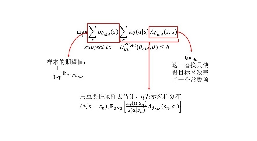
How to replace the advantage values Aθold by the Q values Qθold and only change the objective by a constant?
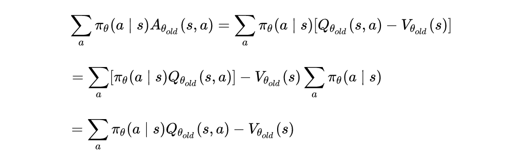
Our optimization problem in Equation (13) is exactly equivalent to the following one, written in terms of expectations:

All that remains is to replace the expectations by sample averages and replace the Q value by an empirical estimate.
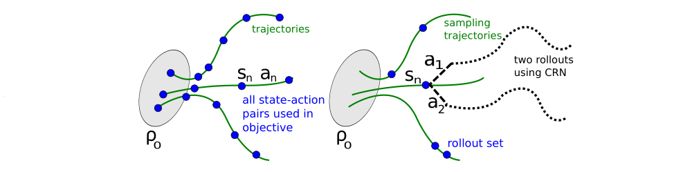
We have two different schemes for performing this estimation. The first sampling scheme, which we call single path, is the one that is typically used for policy gradient estimation, and is based on sampling individual trajectories. The second scheme, which we call vine, involves constructing a rollout set and then performing multiple actions from each state in the rollout set. This method has mostly been explored in the context of policy iteration methods.
6 Practical Algorithm
Here we present two practical policy optimization algorithm based on the ideas above, which use either the single path or vine sampling scheme from the preceding section. The algorithms repeatedly perform the following steps:
-
Use the single path or vine procedures to collect a set of state-action pairs along with Monte Carlo estimates of their Q-values.
-
By averaging over samples, construct the estimated objective and constraint in Equation (14).
-
Approximately solve this constrained optimization problem to update the policy’s parameter vector θ. We use the conjugate gradient (共轭梯度)algorithm followed by a line search, which is altogether only slightly more expensive than computing the gradient itself.
Then we’ll discuss how to efficiently approximately solve the Trust Region Constrained Optimization Problem.
We first approximate the optimization problem. The original objective and constraint equation respect to θ is:

After doing some estimation, we abbreviate it as below:

We approximate l(θ) using Taylor Series up to the first order for l(θ) at θold:
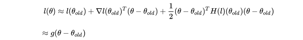
Note that the first term of the right-hand side is 0, the third term is quite small and

Then we approximate kl(θ) using Taylor Series up to the second order for kl(θ) at θold:
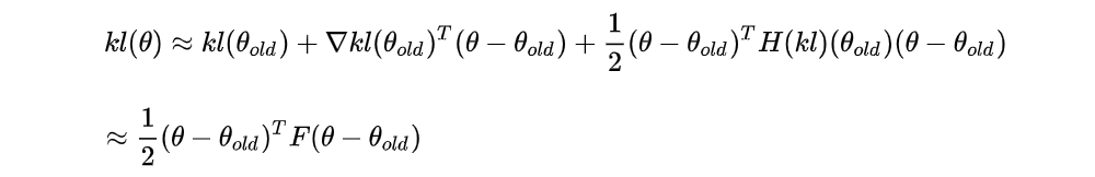
Note that the first term and second term of the right-hand side are both 0,

Until now, the optimization problem has been approximated as:

The method that we’ll describe involves two steps: (1) compute a search direction, using a linear approximation to objective and quadratic approximation to the constraint (as is mentioned above); and (2) perform a line search in that direction, ensuring that we improve the nonlinear objective while satisfying the nonlinear constraint.
The search direction is computed by approximately solving the equation Ax = g, where g is the policy gradient and A is called the Fisher information matrix FIM in the form of a Hessian matrix, i.e., the quadratic approximation to the KL divergence constraint:

where

In large-scale problems, it is prohibitively costly (with respect to computation and memory) to form the full matrix A (or A inverse). However, the conjugate gradient algorithm allows us to approximately solve the equation Ax = b without forming this full matrix, when we merely have access to a function that computes matrix-vector products y → Ay. Appendix C.1 describes the most efficient way to compute matrix-vector products with the averaged Fisher information matrix and arbitrary vectors.
Having computed the search direction

we next need to compute the maximal step length β, such that the θ + βs will satisfy the KL divergence constraint. To do this, let

From this, we obtain

where δ is the desired KL divergence. The term sTAs can be computed through a single Hessian vector product, and it is also an intermediate result produced by the conjugate gradient algorithm.
Last, we use a line search to ensure improvement of the surrogate objective and satisfaction of the KL divergence constraint, both of which are nonlinear in the parameter vector θ (and thus depart from the linear and quadratic approximations used to compute the step). We perform the line search on the objective.

where X[…] equals 0 when its argument is true and +∞ when it is false. Starting with the maximal value of the step length β computed in the previous paragraph, we shrink β exponentially until the objective improves. Without this line search, the algorithm occasionally computes large steps that cause a catastrophic degradation of performance.
Let us briefly summarize the relationship between the theory from Section 3 and the practical algorithm we have described above:
-
The theory justifies optimizing a surrogate objective with a penalty on KL divergence. However, the large penalty coefficient C leads to prohibitively small steps, so we would like to decrease this coefficient. Empirically, it is hard to robustly choose the penalty coefficient, so we use a hard constraint instead of a penalty, with parameter δ (the bound on KL divergence)
-
Replace maximum KL divergence constraint with average KL divergence constraint because the former is hard for numerical optimization and estimation.
-
Our theory ignores estimation error for the advantage function, we omit them for simplicity.
7 Connection with prior work
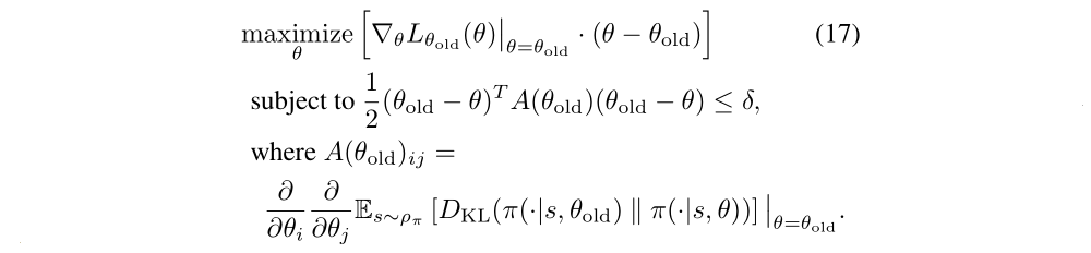
As mentioned in Section 4, our derivation results in a policy update that is related to several prior methods, providing a unifying perspective on a number of policy update schemes. The Natural Policy Gradient can be obtained as a special case of the update in Equation (12) by using a linear approximation to L and a quadratic approximation to the average KL divergence constraint, resulting in the follow problem:
And the update is

where the stepsize 1/λ is typically treated as an algorithm parameter. This differs from our approach, which enforces the constraint at each update. Though this difference might seem subtle, our experiments demonstrate that it significantly improves the algorithm’s performance on larger problems.
We can also obtain the standard policy gradient update by using an L2 constraint or penalty:

The policy iteration update can also be obtained by solving the unconstrained problem
