Paper 2: Proximal Policy Optimization Algorithms (PPO)
Abstract
-
Whereas standard policy gradient methods perform one gradient update per data sample, we propose a novel objective function that enables
multiple epochs of minibatch updates. -
Have some of the benefits of TRPO, but is much simpler to implement, more general, and have better sample complexity (empirically)
-
Outperforms other online policy gradient methods on a collection of benchmark tasks.
1 Introduction
There is room for improvement in developing a method that is scalable (to large models and parallel implementations), data efficient, and robust (i.e., successful on a variety of problems without hyperparameter tuning).
This paper seeks to improve the current state of affairs by introducing an algorithm that attains the data efficiency and reliable performance of TRPO, while using only first order approximation. We propose a novel objective with clipped probability ratios, which forms a pessimistic estimate (i.e., lower bound) of the performance of the policy. To optimize policies, we alternate between sampling data from the policy and performing several epochs of optimization on the sampled data.
2 Background: Policy Optimization
2.1 Policy Gradient Methods
Policy gradient methods work by computing an estimator of the policy gradient and plugging it into a stochastic gradient ascent algorithm. The most commonly used gradient estimator has the form

where πθ is a stochastic policy and Aˆt is an estimator of the advantage function at timestep t. Here, the expectation ˆEt[. . .] indicates the empirical average over a finite batch of samples, in an algorithm that alternates between sampling and optimization.
Implementations that use automatic differentiation software work by constructing an objective function whose gradient is the policy gradient estimator; the estimator ˆg is obtained by differentiating the objective

While it is appealing to perform multiple steps of optimization on this loss using the same trajectory, doing so is not well-justified, and empirically it often leads to destructively large policy updates.
2.2 Trust Region Methods
In TRPO, an objective function (the “surrogate” objective) is maximized subject to a constraint on the size of the policy update. Specifically,
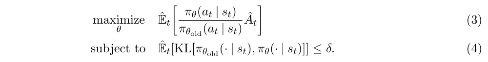
Here, θold is the vector of policy parameters before the update. This problem can efficiently be approximately solved using the conjugate gradient algorithm, after making a linear approximation to the objective and a quadratic approximation to the constraint.
The theory justifying TRPO actually suggests using a penalty instead of a constraint, i.e., solving the unconstrained optimization problem

for some coefficient β. This follows from the fact that a certain surrogate objective (which computes the max KL over states instead of the mean) forms a lower bound (i.e., a pessimistic bound) on the performance of the policy π. TRPO uses a hard constraint rather than a penalty because it is hard to choose a single value of β that performs well across different problems—or even within a single problem, where the the characteristics change over the course of learning. Hence, to achieve our goal of a first-order algorithm that emulates the monotonic improvement of TRPO, experiments show that it is not sufficient to simply choose a fixed penalty coefficient β and optimize the penalized objective Equation (5) with SGD; additional modifications are required.
3. Clipped Surrogate Objective
We denote the probability ratio with

So rt(θold) is equal to 1 and TRPO maximizes a “surrogate” objective

The superscript CPI refers to the conservative policy iteration, where this objective was proposed. Without a constraint, maximization of LCPI would lead to an excessively large policy update; hence, we now consider how to modify the objective, to penalize changes to the policy that move rt(θ) away from 1.
The main objective we propose is the following:

where ε is a hyperparameter, say, ε= 0.2.
The motivation for this objective is as follows. The first term inside the min is LCPI. The second term,

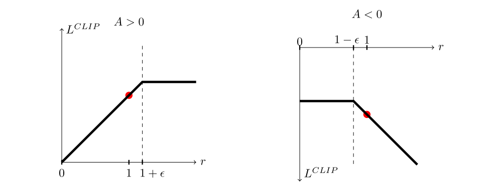
modifies the surrogate objective by clipping the probability ratio, which removes the incentive for moving rt outside of the interval [1 − ε, 1 + ε]. Finally, we take the minimum of the clipped and unclipped objective, so the final objective is a lower bound (i.e., a pessimistic bound) on the unclipped objective. With this scheme, we only ignore the change in probability ratio when it would make the objective improve, and we include it when it makes the objective worse. Note that

to first order around θold (i.e., where r = 1), however, they become different as θ moves away from θold. The following figure plots a single term (i.e., a single t) in LCLIP; note that the probability ratio r is clipped at 1 − ε or 1 + ε depending on whether the advantage is positive or negative.
4 Adaptive KL Penalty Coefficient
Another approach, which can be used as an alternative to the clipped surrogate objective, or in addition to it, is to use a penalty on KL divergence, and to adapt the penalty coefficient so that we achieve some target value of the KL divergence dtarg each policy update. In our experiments, we found that the KL penalty performed worse than the clipped surrogate objective, however, we’ve included it here because it’s an important baseline.
In the simplest instantiation of this algorithm, we perform the following steps in each policy update:
-
Using several epochs of minibatch SGD, optimize the KL-penalized objective

-
Compute

The updated β is used for the next policy update. With this scheme, we occasionally see policy updates where the KL divergence is significantly different from dtarg, however, these are rare, and β quickly adjusts. The parameters 1.5 and 2 above are chosen heuristically, but the algorithm is not very sensitive to them. The initial value of β is a another hyperparameter but is not important in practice because the algorithm quickly adjusts it.
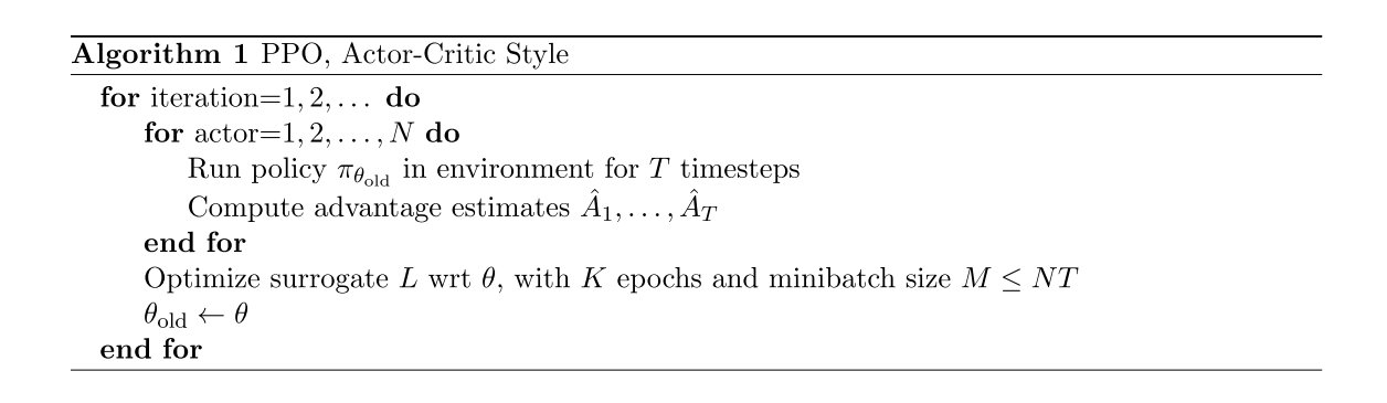
5 Algorithm
The surrogate losses from the previous sections can be computed and differentiated with a minor change to a typical policy gradient implementation. For implementations that use automatic differentiation, one simply constructs the loss LCLIP or LKLPEN instead of LPG, and one performs multiple steps of stochastic gradient ascent on this objective.
Most techniques for computing variance-reduced advantage-function estimators make use a learned state-value function V(s). If using a neural network architecture that shares parameters between the policy and value function, we must use a loss function that combines the policy surrogate and a value function error term. This objective can further be augmented by adding an entropy bonus to ensure sufficient exploration. Combining these terms, we obtain the following objective, which is (approximately) maximized each iteration:

where c1, c2 are coefficients, and S denotes an entropy bonus, and the second term in the right-hand side is a squared-error loss:

One style of policy gradient implementation runs the policy for T timesteps (where T is much less than the episode length), and uses the collected samples for an update. This style requires an advantage estimator that does not look beyond timestep T. The estimator is

where t specifies the time index in [0, T], within a given length-T trajectory segment. Generalizing this choice, we can use a truncated version of generalized advantage estimation, which reduces to Equation (10) when λ = 1:

A proximal policy optimization (PPO) algorithm that uses fixed-length trajectory segments is shown below. Each iteration, each of N (parallel) actors collect T timesteps of data. Then we construct the surrogate loss on these NT timesteps of data, and optimize it with minibatch SGD (or usually for better performance, Adam), for K epochs.