Paper 8: Playing FPS Games with Deep Reinforcement Learning (ViZDoom)
Abstract
-
We present the first architecture to tackle 3D environments in first-person shooter games, that involve partially observable states.
-
Our DRL methods only utilize visual input for training, we present a method to augment these models to exploit game feature information such as the presence of enemies or items, during the training phase.
-
Our model is trained to simultaneously learn these features along with minimizing a Q-learning objective, which is shown to dramatically improve the training speed and performance of our agent.
-
Our architecture is also modularized to allow different models to be independently trained for different phases of the game.
1 Introduction
There’s a limitation in all of the current applications in their assumption of having the full knowledge of the current state of the environment, which is usually not true in real-world scenarios. In the case of partially observable states, the learning agent needs to remember previous states in order to select optimal actions.
Recently, there have been attempts to handle partially observable states in deep reinforcement learning by introducing recurrency in Deep Q-networks. The use of RNN (or LSTM) is effective in scenarios with partially observable states due to its ability to remember information for an arbitrarily long amount of time.
Previous methods have usually been applied to 2D environments that hardly resemble the real world. In this paper, we tackle the task of playing a First-Person-Shooting (FPS) game in a 3D environment. This task is much more challenging than playing most Atari games as it involves a wide variety of skills, such as navigating through a map, collecting items, recognizing and fighting enemies, etc. Furthermore, states are partially observable, and the agent navigates a 3D environment in a first-person perspective, which makes the task more suitable for real-world robotics applications.
We present an AI-agent for playing deathmatches in FPS games using only the pixels on the screen. A deathmatch is a scenario in FPS games where the objective is to maximize the number of kills by a player/agent. Our agent divides the problem into two phases:
-
Navigation(exploring the map to collect items and find enemies) -
Action(fighting enemies when they are observed)
We use separate networks for each phase of the game. The agent infers high-level game information, such as the presence of enemies on the screen, to decide its current phase and to improve its performance.
We also introduce a method for co-training a DQN with game features, which turned out to be critical in guiding the convolutional layers of the network to detect enemies. We show that co-training significantly improves the training speed and performance of the model.
2 Background
A brief summary of the DQN and DRQN models.
2.1 Deep Q-Networks
2.2 Deep Recurrent Q-Networks
The above model assumes that at each step, the agent receives a full observation st of the environment - as opposed to games like Go, Atari games actually rarely return a full observation, since they still contain hidden variables, but the current screen buffer is usually enough to infer a very good sequence of actions. But in partially observable environments, the agent only receives an observation ot of the environment which is usually not enough to infer the full state of the system. A FPS game like DOOM, where the agent field of view is limited to 90 centered around its position, obviously falls into this category.
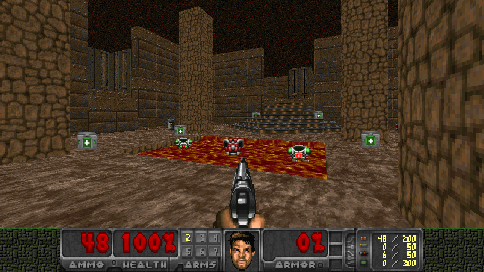
Figure 1: A screenshot of Doom
To deal with such environments, someone introduced the Deep Recurrent Q-Networks (DRQN), which does not estimate Q(st, at), but Q(ot, ht−1, at), where ht is an extra input returned by the network at the previous step, that represents the hidden state of the agent. A recurrent neural network like a LSTM can be implemented on top of the normal DQN model to do that. In that case, ht=LSTM(ht−1, ot), and we estimate Q(ht, at). Our model is built on top of the DRQN architecture.
3 Model
Our first approach to solving the problem was to use a baseline DRQN model. Although this model achieved good performance in relatively simple scenarios (where the only available actions were to turn or attack), it did not perform well on deathmatch tasks. The resulting agents were firing at will, hoping for an enemy to come under their lines of fire. Giving a penalty for using ammo(弹药)did not help: with a small penalty, agents would keep firing, and with a big one they would just never fire.
3.1 Game feature augmentation
We reason that the agents were not able to accurately detect enemies. The ViZDoom environment gives access to internal variables generated by the game engine. We modified the game engine so that it returns, with every frame, information about the visible entities. Therefore, at each step, the network receives a frame, as well as a Boolean value for each entity, indicating whether this entity appears in the frame or not (an entity can be an enemy, a health pack, a weapon, ammo, etc). Although this internal information is not available at test time, it can be exploited during training. We modified the DRQN architecture to incorporate this information and to make it sensitive to game features.
In the initial model, the output of the CNN is given to a LSTM that predicts a score for each action based on the current frame and its hidden state. We added two fully-connected layers of size 512 and k connected to the output of the CNN, where k is the number of game features we want to detect. At training time, the cost of the network is a combination of the normal DRQN cost and the cross-entropy loss. Note that the LSTM only takes as input the CNN output, and is never directly provided with the game features.
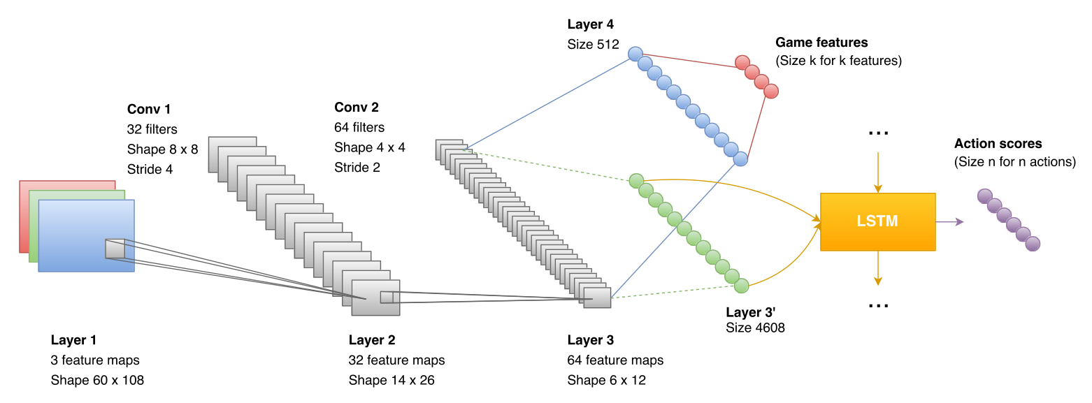
Figure 2: An illustration of the architecture of our model
Although a lot of game information was available, we only used an indicator about the presence of enemies on the current frame. Adding this game feature dramatically improved the performance of the model on every scenario we tried.
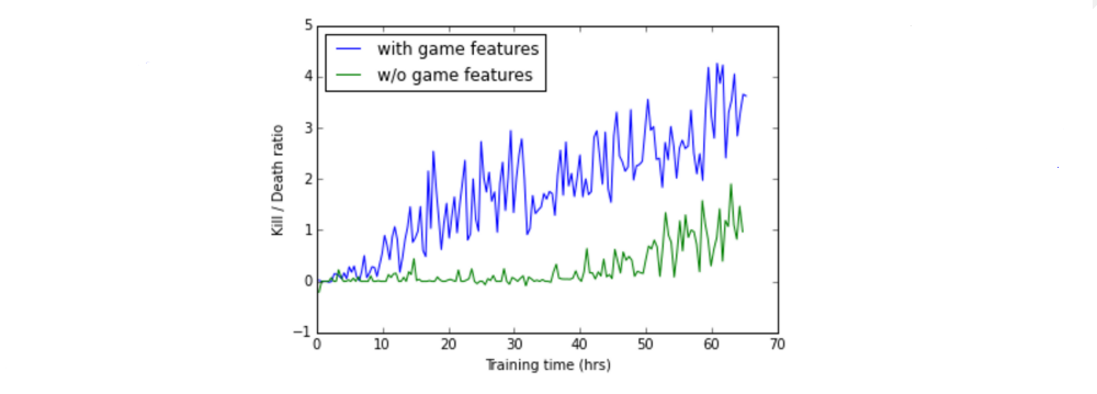
Figure 3: The performance of the DRQN with and without the game features
We explored other architectures to incorporate game features, such as using a separate network to make predictions and reinjecting the predicted features into the LSTM, but this did not achieve results better than the initial baseline, suggesting that sharing the convolutional layers is decisive in the performance of the model. Jointly training the DRQN model and the game feature detection allows the kernels of the convolutional layers to capture the relevant information about the game. In our experiments, it only takes a few hours for the model to reach an optimal enemy detection accuracy of 90%. After that, the LSTM is given features that often contain information about the presence of enemy and their positions, resulting in accelerated training.
Augmenting a DRQN model with game features is straightforward. However, the above method can not be applied easily to a DQN model. In a DQN model, the network receives k frames at each time step, and will have to predict whether some features appear in the last frame only, independently of the content of the k−1 previous frames. Convolutional layers do not perform well in this setting.
3.2 Divide and conquer(分而治之)
The deathmatch task is typically divided into two phases, one involves exploring the map to collect items and to find enemies, and the other consists in fighting enemies. We call these phases the navigation and action phases. Having two networks work together, each trained to act in a specific phase of the game should naturally lead to a better overall performance. Current DQN models do not allow for the combination of different networks optimized on different tasks. However, the current phase of the game can be determined by predicting whether an enemy is visible in the current frame (action phase) or not (navigation phase), which can be inferred directly from the game features present in the proposed model architecture.
There are various advantages of splitting the task into two phases and training a different network for each phase.
-
First, this
makes the architecture modular and allows different models to be trained and tested independently for each phase. Both networks can be trained in parallel, which makes the training much faster as compared to training a single network for the whole task. -
Furthermore, the navigation phase only requires three actions (move forward, turn left and turn right), which dramatically
reduces the number of state-action pairs required to learn the Q-function, and makes the training much faster. -
More importantly, using two networks also
mitigates(缓和)“camper” behavior, i.e. tendency to stay in one area of the map and wait for enemies, which was exhibited by the agent when we tried to train a single DQN or DRQN for the deathmatch task.
We trained two different networks for our agent. We used a DRQN augmented with game features for the action network, and a simple DQN for the navigation network. During the evaluation, the action network is called at each step. If no enemies are detected in the current frame, or if the agent does not have any ammo left, the navigation network is called to decide the next action. Otherwise, the decision is given to the action network.
4 Training (common techniques)
4.1 Reward Shaping
The score in the deathmatch scenario is defined as the number of frags, i.e. number of kills minus number of suicides. If the reward is only based on the score, the replay table is extremely sparse w.r.t state-action pairs having non-zero rewards, which makes it very difficult for the agent to learn favorable actions. Moreover, rewards are extremely delayed and are usually not the result of a specific action: getting a positive reward requires the agent to explore the map to find an enemy and accurately aim and shoot it with a slow projectile rocket. The delay in reward makes it difficult for the agent to learn which set of actions is responsible for what reward.
To tackle the problem of sparse replay table and delayed rewards, we introduce reward shaping, i.e. the modification of reward function to include small intermediate rewards to speed up the learning process. In addition to positive reward for kills and negative rewards for suicides, we introduce the following intermediate rewards for shaping the reward function of the action network:
-
positive reward for object pickup (health, weapons and ammo)
-
negative reward for loosing health (attacked by enemies or walking on lava)
-
negative reward for shooting, or loosing ammo
We used different rewards for the navigation network. Since it evolves on a map without enemies and its goal is just to gather items, we simply give it a positive reward when it picks up an item, and a negative reward when it’s walking on lava(岩浆). We also found it very helpful to give the network a small positive reward proportional to the distance it travelled since the last step. That way, the agent is faster to explore the map, and avoids turning in circles.
4.2 Frame Skip
The agent only receives a screen input every k+1 frames, where k is the number of frames skipped between each step. The action decided by the network is then repeated over all the skipped frames. A higher frame-skip rate accelerates the training, but can hurt the performance. Typically, aiming at an enemy sometimes requires to rotate by a few degrees, which is impossible when the frame skip rate is too high, even for human players, because the agent will repeat the rotate action many times and ultimately rotate more than it intended to. A frame skip of k=4 turned out to be the best trade-off.
4.3 Sequential Updates
To perform the DRQN updates, we use a different approach from the one presented by the original paper. A sequence of n observations o1, o2, …, on is randomly sampled from the replay memory, but instead of updating all action-states in the sequence, we only consider the ones that are provided with enough history. Indeed, the first states of the sequence will be estimated from an almost non-existent history (since h0 is reinitialized at the beginning of the updates), and might be inaccurate. As a result, updating them might lead to imprecise updates.
To prevent this problem, errors from states o1…oh, where h is the minimum history size for a state to be updated, are not backpropagated through the network. Errors from states oh+1..on−1 will be backpropagated, on only being used to create a target for the on−1 action-state. An illustration of the updating process is presented in Figure 4, where h=4 and n=8.
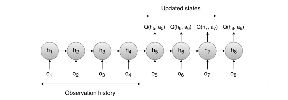
Figure 4: DRQN updates in the LSTM
As shown in the figure, only the scores of the actions taken in states 5, 6 and 7 will be updated. First four states provide a more accurate hidden state to the LSTM, while the last state provide a target for state 7.
In all our experiments, we set the minimum history size to 4, and we perform the updates on 5 states. Increasing the number of updates leads to high correlation in sampled frames, violating the DQN random sampling policy, while decreasing the number of updates makes it very difficult for the network to converge to a good policy.
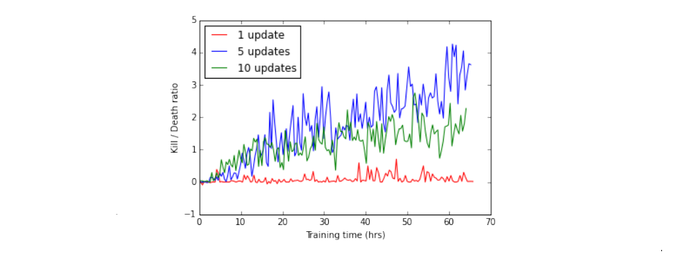
Figure 5: The importance of selecting an appropriate number of
updates