Paper 16: IMPALA: Scalable Distributed Deep-RL with Importance Weighted Actor-Learner Architectures
Abstract
-
We have developed a new distributed agent IMPALA (Importance Weighted Actor-Learner Architecture) that not only uses resources more efficiently in single-machine training but also scales to thousands of machines without sacrificing data efficiency or resource utilization.
-
We achieve stable learning at high throughput(吞吐量)by combining decoupled acting and learning with a novel off-policy correction method called V-trace.
-
Our results show that IMPALA is able to achieve better performance than previous agents with less data, and crucially exhibits positive transfer between tasks as a result of its multi-task approach.
1 Introduction
We are interested in developing new methods capable of mastering a diverse set of tasks simultaneously as well as environments suitable for evaluating such methods.
One of the main challenges in training a single agent on many tasks at once is scalability. Training A3C and UNREAL on tens of domains at once is too slow to be practical.
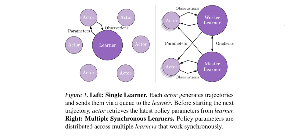
We propose the IMPALA shown in Figure 1.
IMPALA is capable of scaling to thousands of machines without sacrificing training stability or data efficiency. Unlike the popular A3C-based agents, in which workers communicate gradients with respect to the parameters of the policy to a central parameter server, IMPALA actors communicate trajectories of experience to a centralised learner. Since the learner in IMPALA has access to full trajectories of experience we use a GPU to perform updates on mini-batches of trajectories while aggressively parallelising all time independent operations. This type of decoupled architecture can achieve very high throughput. However, because the policy used to generate a trajectory can lag behind the policy on the learner by several updates at the time of gradient calculation, learning becomes off-policy. Therefore, we introduce the V-trace off-policy actor-critic algorithm to correct for this harmful discrepancy.
With the scalable architecture and V-trace combined, IMPALA achieves exceptionally high data throughput rates of 250,000 frames per second, making it over 30 times faster than single-machine A3C. Crucially, IMPALA is also more data efficient than A3C based agents and more robust to hyperparameter values and network architectures, allowing it to make better use of deeper neural networks.
3 IMPALA
IMPALA uses an actor-critic setup to learn a policy π and a baseline function Vπ. The process of generating experiences is decoupled from learning the parameters of π and Vπ. The architecture consists of a set of actors, repeatedly generating trajectories of experience, and one or more learners that use the experiences sent from actors to learn π off-policy.
At the beginning of each trajectory, an actor updates its own local policy µ to the latest learner policy π and runs it for n steps in its environment. After n steps, the actor sends the trajectory of states, actions and rewards together with the corresponding policy distributions µ(at|xt) and initial LSTM state to the learner through a queue. The learner then continuously updates its policy π on batches of trajectories, each collected from many actors. This simple architecture enables the learner(s) to be accelerated using GPUs and actors to be easily distributed across many machines. However, the learner policy π is potentially several updates ahead of the actor’s policy µ at the time of update, therefore there is a policy-lag between the actors and learner(s). V-trace corrects for this lag to achieve extremely high data throughput while maintaining data efficiency. Using an actor-learner architecture, provides fault tolerance like distributed A3C but often has lower communication overhead since the actors send observations rather than parameters/gradients.
IMPALA can be used with distributed set of learners to train large neural networks efficiently as shown in Figure 1. Parameters are distributed across the learners and actors retrieve the parameters from all the learners in parallel while only sending observations to a single learner. IMPALA use synchronised parameter update which is vital to maintain data efficiency when scaling to many machines.
3.1 Efficiency Optimizations
Since the learner in IMPALA performs updates on entire batches of trajectories, it is able to parallelize more of its computations than an online agent like A3C. As an example, a typical deep RL agent features a CNN followed by a LSTM and a fully connected output layer after the LSTM. An IMPALA learner applies the CNN to all inputs in parallel by folding the time dimension into the batch dimension. Similarly, it also applies the output layer to all time steps in parallel once all LSTM states are computed. This optimization increases the effective batch size to thousands. LSTM-based agents also obtain significant speedups on the learner by exploiting the network structure dependencies and operation fusion.
Finally, we also make use of several off the shelf optimizations available in TensorFlow such as preparing the next batch of data for the learner while still performing computation, compiling parts of the computational graph with XLA (a TensorFlow Just-In-Time compiler) and optimizing the data format to get the maximum performance from the cuDNN framework.
4 V-trace Off-policy
Off-policy learning is important in the decoupled distributed actor-learner architecture because of the lag between when actions are generated by the actors and when the learner estimates the gradient. To this end, we introduce a novel off-policy actor-critic algorithm for the learner, called V-trace.
The goal of an off-policy RL algorithm is to use trajectories generated by some policy µ, called the behaviour policy, to learn the value function Vπ of another policy π (possibly different from µ), called the target policy.
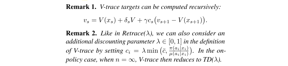
4.1 V-trace target
We define the n-steps V-trace target for V(xs), our value approximation at state xs, as:

where

is a temporal difference for V, and

and

are truncated importance sampling (IS) weights. We make use of the notation

for s = t. In addition we assume that the truncation levels are such that ¯ρ ≥ ¯c.
Notice that in the on-policy case (when π = µ), and assuming that ¯c ≥ 1, then all ci = 1 and ρt = 1, thus (1) rewrites

which is the on-policy n-steps Bellman target. Thus in the on-policy case, V-trace reduces to the on-policy n-steps Bellman update. This property allows one to use the same algorithm for off- and on-policy data.
Notice that the (truncated) IS weights ci and ρt play different roles. The weight ρt appears in the definition of the temporal difference δtV and defines the fixed point of this update rule. In a tabular case, where functions can be perfectly represented, the fixed point of this update (i.e., when V(xs) = vs for all states), characterized by δtV being equal to zero in expectation (under µ), is the value function Vπ¯ρ of some policy π¯ρ, defined by

So when ¯ρ is infinite (i.e. no truncation of ρt), then this is the value function Vπ of the target policy. However if we choose a truncation level ¯ρ < ∞, our fixed point is the value function Vπ¯ρ of a policy π¯ρ which is somewhere between µ and π. At the limit when ¯ρ is close to zero, we obtain the value function of the behaviour policy Vµ. In Appendix A we prove the contraction of a related V-trace operator and the convergence of the corresponding online V-trace algorithm.
The weights ci are similar to the “trace cutting” coefficients a temporal difference δtV observed at time t impacts the in Retrace. Their product cs . . . ct−1 measures how much update of the value function at a previous time s. The more dissimilar π and µ are (the more off-policy we are), the larger the variance of this product. We use the truncation level ¯c as a variance reduction technique. However notice that this truncation does not impact the solution to which we converge (which is characterized by ¯ρ only).
Thus we see that the truncation levels ¯c and ¯ρ represent different features of the algorithm: ¯ρ impacts the nature of the value function we converge to, whereas ¯c impacts the speed at which we converge to this function.
4.2 Actor-Critic Algorithm
In the off-policy setting that we consider, we can use an IS weight between the policy being evaluated π¯ρ and the behaviour policy µ, to update our policy parameter in the direction of

where

is an estimate of Qπ¯ρ(xs, as) built from the V-trace estimate vs+1 at the next state xs+1. In order to reduce the variance of the policy gradient estimate (4), we usually subtract from qs a state-dependent baseline, such as the current value approximation V(xs).
Finally notice that (4) estimates the policy gradient for π¯ρ which is the policy evaluated by the V-trace algorithm when using a truncation level ¯ρ. However assuming the bias Vπ¯ρ − Vπ is small (e.g. if ¯ρ is large enough) then we can expect qs to provide us with a good estimate of Qπ(xs, as). Taking into account these remarks, we derive the following canonical V-trace actor-critic algorithm.
V-trace Actor-Critic Algorithm
Consider a parametric representation Vθ of the value function and the current policy πω. Trajectories have been generated by actors following some behaviour policy µ. The V-trace targets vs are defined by (1). At training time s, the value parameters θ are updated by gradient descent on the l2 loss to the target vs, i.e., in the direction of

and the policy parameters ω in the direction of the policy gradient:

In order to prevent premature convergence we may add an entropy bonus, like in A3C, along the direction

The overall update is obtained by summing these three gradients rescaled by appropriate coefficients, which are hyper-parameters of the algorithm.
5 Experiments
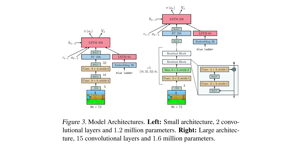
For all the experiments we have used two different model architectures: a shallow model with an LSTM before the policy and value and a deeper residual model. For tasks with a language channel we used an LSTM with text embeddings as input.