Paper 26: GA3C: GPU-based A3C for Deep Reinforcement Learning
Github: https://github.com/NVlabs/GA3C.
Abstract
-
We introduce and analyze the computational aspects of a hybrid CPU/GPU implementation of the A3C algorithm.
-
Our analysis concentrates on the critical aspects to leverage the GPU’s computational power, including the introduction of a system of queues and a dynamic scheduling strategy, potentially helpful for other asynchronous algorithms as well. We also show the potential for the use of larger DNN models on a GPU.
-
Our TensorFlow implementation achieves a significant speed up compared to our CPU-only implementation, and it will be made publicly available to other researchers.
1 Introduction
A3C dispenses with the large replay memory of previous approaches by stabilizing learning with updates from several concurrently playing agents. For the task of learning to play an Atari game from raw screen inputs, with a proper learning rate, A3C learns better strategies on a 16-core CPU than previous methods trained for the same amount of time on a GPU.
Our study sets aside the learning aspects of recent work and instead delves into computational issues of deep RL. Computational complexities are numerous, but largely center on a common factor: RL has an inherently sequential aspect since the training data is generated during learning. The DNN is constantly queried to guide agents whose gameplay in turn feeds DNN training. Training batches are commonly small and must be efficiently shepherded from the agents and simulator to the DNN trainer. While DQN methods maintain a large set of past experiences to smooth over some of these issues, A3C feeds agent experiences directly into training with little delay. When using a GPU, the mix of small DNN architectures and small batch sizes can severely underutilize(未充分利用)computational resources.
To systematically investigate these issues, we implement both CPU and GPU versions of A3C in TensorFlow, optimizing each for efficient system utilization and to match published scores in the Atari 2600 environment. We analyze a variety of “knobs” in the system and demonstrate effective automatic tuning during training. The GPU implementation (GA3C) learns substantially faster (up to ∼ 90× for large DNNs) than its CPU counterpart. While we focus on the A3C architecture, we hope this analysis will be helpful for researchers and framework developers working on the next generation of deep RL methods.
2 Hybrid CPU/GPU A3C (GA3C)
In A3C, multiple agents play concurrently and optimize a DNN controller using asynchronous gradient descent. Similar to other asynchronous methods, the DNN weights are stored in a central parameter server. Agents calculate gradients and send updates to the server, which propagates new weights to the agents between updates to maintain a shared policy. The original implementation of A3C uses 16 agents on a 16 core CPU and takes 1 − 4 days to learn how to play an Atari game.
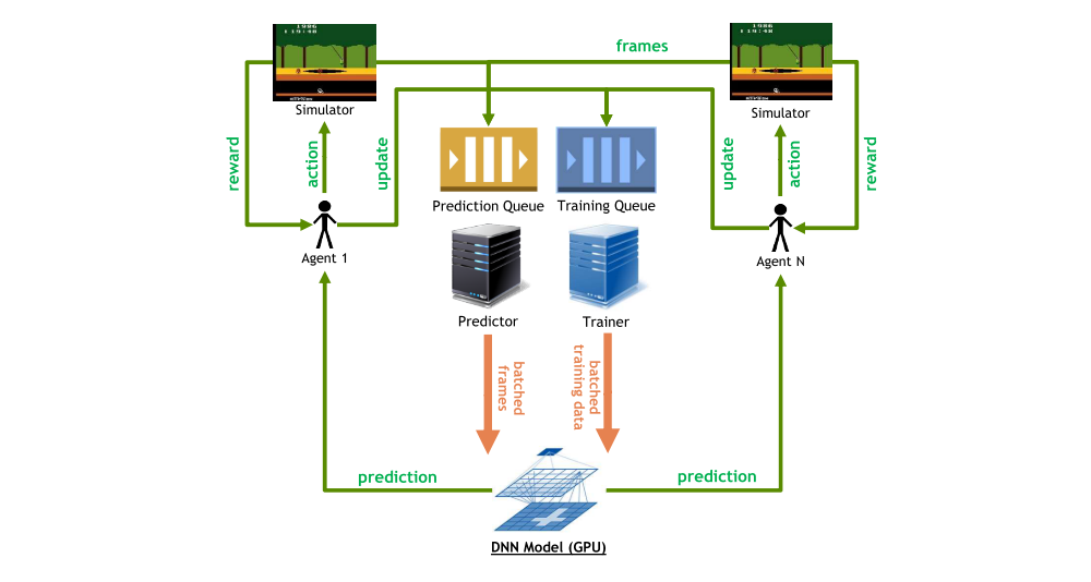
For our performance profiling, we implement a hybrid GPU-CPU architecture (GA3C) as depicted in the following figure. The primary components are a traditional DNN model with training and prediction on a GPU, as well as a multi-process, multi-threaded CPU architecture with the following components:
-
Agentis a process interacting with the simulation environment by actions chosen according to the learned policy and gathering experiences for further training. Similar to A3C, multiple concurrent agents run independent instances of the environment in GA3C. Unlike the original, each agent does not have its own copy of the model. Instead it queues policy requests in a Prediction Queue before each action, and periodically submits a batch of input/reward experiences to a Training Queue. -
Predictoris a thread which dequeues as many prediction requests as are immediately available and batches them into a single inference query to the DNN model on the GPU. When predictions are completed, the predictor returns the requested policy to each respective waiting agent. To hide latency, one or more predictors may act concurrently. -
Traineris a thread which dequeues training batches submitted by agents and submits them to the GPU for model updates. While GPU utilization can be increased by grouping training batches among several agents, we found this can lead to slower convergence because fewer updates are applied to the network. Multiple trainers may run in parallel to hide latency.
This architecture exposes numerous tradeoffs for efficiency tuning.
-
Increasing the number of predictors,
NP, allows faster fetching of prediction queries, but leads to smaller prediction batches, resulting in multiple data transfers and overall lower GPU utilization. -
A larger number of trainers,
NT, potentially leads to more frequent updates to the model, but an overhead is paid when too many trainers occupy the GPU while predictors cannot access it. -
Lastly, increasing the number of agents,
NA, ideally generates more training experiences while hiding prediction latency. However we expect diminishing returns from unnecessary context switching overheads after exceeding some threshold dependent on the number of CPU cores. Additional agents will tend to fill the training queue, introducing an additional time delay between agent experiences and corresponding model updates, threatening model convergence.
In short, NT, NP, and NA encapsulate many of the complex dynamics in recent deep RL training.
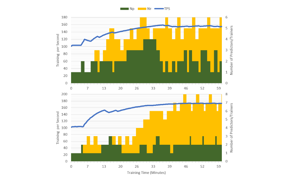
When studying various settings for NT, NP and NA, we measure their effects on resource utilization and learning speed. Training per second (TPS) is a measurement of the rate at which we remove batches from the training queue, which corresponds to the rate of model updates. Given a fixed learning rate and agent batch size, updates directly drive learning and convergence. Another metric is predictions per second (PPS), the rate of issuing prediction queries from the prediction queue, which maps to the combined rate of gameplay among all agents. Notice that in A3C a model update occurs every time an agent plays TMAX=5 actions. Hence, in a balanced configuration, PPS≈TPS×TMAX. Since each action is repeated four times, the number of frames per second is 4×PPS.
Setting NP, NT and NA to maximize TPS also depends on the amount of computation to run the simulation environment, the size of the DNN, the available hardware, and any shared load on the system. As a rule of thumb, we match agents NA to the number of available CPU cores, with predictors and trainers NP = NT = 2. Furthermore, we propose an annealing(退火)process to configure the system dynamically. Every minute we randomly change NP and NT by ±1, monitoring change in TPS to accept or reject the new setting. This way, the optimal configuration is automatically identified in a reasonable time for different environments or systems, even in the case of unpredictable external factors. The following figure shows two cases of the automatic adjustment procedure on a real system: starting from a sub-optimal configuration (NA = 32, NT = NP = 1), the TPS—and, consequently, also PPS—increases while NT and NP converge towards their optimal values.