Paper 28: Distributed Distributional Deterministic Policy Gradients (D4PG)
Abstract
-
This work adopts the very successful distributional perspective on RL and adapts it to the continuous control setting.
-
We combine this within a distributed framework for off-policy learning in order to develop what we call the Distributed Distributional Deep Deterministic Policy Gradient algorithm, D4PG.
-
We also combine this technique with a number of additional, simple improvements such as the use of N-step returns and prioritized experience replay.
-
Experimentally we examine the contribution of each of these individual components, and show how they interact, as well as their combined contributions.
1 Introduction
In this work we consider a number of modifications to the DDPG algorithm. This algorithm has several properties that make it ideal for the enhancements we consider, which is at its core an off-policy actor-critic method. In particular, the policy gradient used to update the actor network depends only on a learned critic. This means that any improvements to the critic learning procedure will directly improve the quality of the actor updates. In this work we utilize a distributional version of the critic update which provides a better, more stable learning signal. Such distributions model the randomness due to intrinsic factors, among these is the inherent uncertainty imposed by function approximation in a continuous environment. We will see that using this distributional update directly results in better gradients and hence improves the performance of the learning algorithm.
Due to the fact that DDPG is capable of learning off-policy it is also possible to modify the way in which experience is gathered. In this work we utilize this fact to run many actors in parallel, all feeding into a single replay table. This allows us to seamlessly distribute the task of gathering experience, which we implement using the ApeX framework. This results in significant savings in terms of wall-clock time for difficult control tasks. We will also introduce a number of small improvements to the DDPG algorithm, and in our experiments will show the individual contributions of each component. Finally, D4PG obtains state-of-the-art performance across a wide variety of control tasks, including hard manipulation and locomotion tasks.
2 Background
The state-action value function is defined as
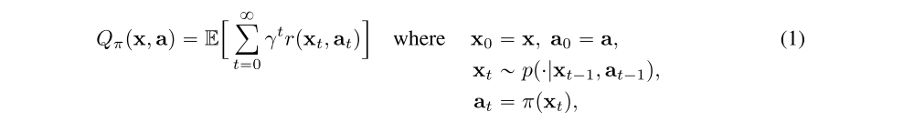
we will consider a parameterized policy πθ and maximize the expected value of this policy by optimizing

By making use of the deterministic policy gradient theorem one can write the gradient of this objective as

While the exact gradient given by (2) assumes access to the true value function of the current policy, we can instead approximate this quantity with a parameterized critic Qw(x, a). By introducing the Bellman operator

we can minimize the TD error. Typically the TD error will be evaluated under separate target policy and value networks, in order to stabilize learning. By taking the two-norm of this error we can write the resulting loss as

Finally, by training a neural network policy using the deterministic policy gradient in (2) and training a deep neural to minimize the TD error in (4) we obtain the DDPG algorithm. Here a sample-based approximation to these gradients is employed by using data gathered in some replay table.
3 Distributed Distributional DDPG
The approach taken in this work starts from the DDPG algorithm and includes a number of enhancements. These extensions, which we will detail in this section, include a distributional critic update, the use of distributed parallel actors, N-step returns, and prioritization of the experience replay.
First, and perhaps most crucially, we consider the inclusion of a distributional critic. In order to introduce the distributional update we first revisit (1) in terms of the return as a random variable Zπ, such that Qπ(x, a) is equal to the expectation of Zπ(x, a). The distributional Bellman operator can be defined as

where equality is with respect to the probability law of the random variables; note that this expectation is taken with respect to distribution of Z as well as the transition dynamics.
While the definition of this operator looks very similar to the canonical Bellman operator defined in (3), it differs in the types of functions it acts on. The distributional variant takes functions which map from state-action pairs to distributions, and returns a function of the same form. In order to use this function within the context of the actor-critic architecture introduced above, we must parameterize this distribution and define a loss similar to that of Equation 4. We will write the loss as

for some metric d that measures the distance between two distributions. Two components that can have a significant impact on the performance of this algorithm are the specific parameterization used for Zw and the metric d used to measure the distributional TD error. In the experiments that follow we will use the Categorical distribution detailed in that section.
We can complete this distributional policy gradient algorithm by including the action-value distribution inside the actor update from Equation 2. This is done by taking the expectation with respect to the action-value distribution, i.e.

As before, this update can be empirically evaluated by replacing the outer expectation with a sample-based approximation.
Next, we consider a modification to the DDPG update which utilizes N-step returns when estimating the TD error. This can be seen as replacing the Bellman operator with an N-step variant

where the expectation is with respect to the N-step transition dynamics. N-step returns are widely used in the context of many policy gradient algorithms as well as Q-learning variants. This modification can be applied analogously to the distributional Bellman operator in order to make use of it when updating the distributional critic.
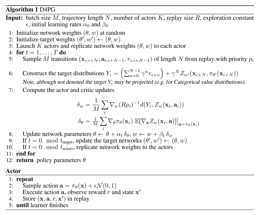
Finally, we also modify the standard training procedure in order to distribute the process of gathering experience. Note from Equations (2,4) that the actor and critic updates rely entirely on sampling from some state-visitation distribution ρ. We can parallelize this process by using K independent actors, each writing to the same replay table. A learner process can then sample from some replay table of size R and perform the necessary network updates using this data. Additionally sampling can be implemented using non-uniform priorities pi. Note that this requires the use of importance sampling, implemented by weighting the critic update by a factor of 1/Rpi. We implement this procedure using the ApeX framework and refer the reader there for more details.
Algorithm pseudocode for the D4PG algorithm which includes all the above-mentioned modifications can be found in Algorithm 1. Here the actor and critic parameters are updated using stochastic gradient descent with learning rates, αt and βt respectively, which are adjusted online using ADAM. While this pseudocode focuses on the learning process, also shown is pseudocode for actor processes which in parallel fill the replay table with data.
4 Result
For algorithms in these experiments we consider actor and critic architectures of the form given in the following figure.
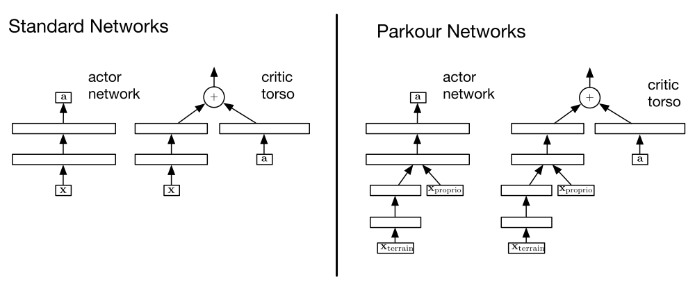
Architectural variants used for each domain
The left-most set illustrates the actor network and critic torso(躯干)used for the standard control and manipulation domains. The full critic architecture is completed by feeding the output of the critic torso into a relevant distribution, e.g. the categorical distribution, as defined in Section A. The right half of the figure similarly illustrates the architecture used by the parkour(跑酷)domains.
Section A: Distributions and Losses
In this section we consider two potential parameterized distributions for D4PG. Parameterized distributions, in this framework, are implemented as a neural network layer mapping the output of the critic torso to the parameters of a given distribution (e.g. mean and variance). In what follows we will detail the distributions and their corresponding losses.

Output layers corresponding to different distribution parameterizations
From left to right these include the Categorical, Mixture of Gaussians, and finally the standard scalar value function.
Categorical: We first consider the categorical parameterization, a layer whose parameters are the logits ωi of a discrete-valued distribution defined over a fixed set of atoms zi. This distribution has hyperparameters for the number of atoms l, and the bounds on the support (Vmin, Vmax). Given these,

corresponds to the distance between atoms, and zi = Vmin + i∆ gives the location of each atom. We can then define the action-value distribution as

Observe that this distributional layer simply corresponds to a linear layer from the critic torso to the logits ω, followed by a softmax activation.
However, this distribution is not closed under the Bellman operator defined earlier, due to the fact that adding and scaling these values will no longer lie on the support defined by the atoms. This support is explicitly defined by the (Vmin, Vmax) hyperparameters. As a result we instead use a projected version of the distributional Bellman operator, see Appendix B for more details. Letting p’ be the probabilities of the projected distributional Bellman operator ΦTπ applied to some target distribution Ztarget, we can write the loss in terms of the cross-entropy

Mixture of Gaussians: We can also consider parameterizing the action-value distribution using a mixture of Gaussians; here the random variable Z has density given by

Thus, the distribution layer maps, through a linear layer, from the critic torso to the mixture weight ωi, mean µi, and variance σi2 for each mixture component. We can then specify a loss corresponding to the cross-entropy portion of the KL divergence between two distributions. Given a sample transition (x, a, r, x’) we can take samples from the target density zj ~ ptarget and approximate the cross-entropy term using

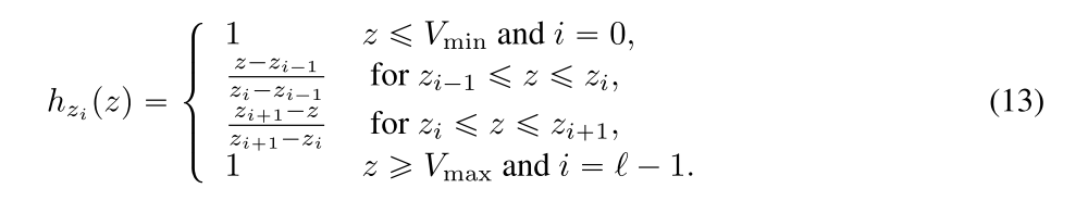
B Categorical Projection Operator
The categorical parameterized distribution has finite support. Thus, the result of applying the distributional Bellman equation will generally not coincide with this support. Therefore, some projection step is required before minimizing the cross-entropy. The categorical projection is given by

where h is a piecewise linear ‘hat’ function,