Paper 30: High-dimensional Continuous Control using Generalized Advantage Estimation (GAE)
Abstract
-
The two main challenges in policy gradient methods are the large number of samples typically required, and the difficulty of obtaining stable and steady improvement despite the nonstationarity of the incoming data.
-
We address the first challenge by using value functions to substantially reduce the variance of policy gradient estimates at the cost of some bias, with an exponentially-weighted estimator of the advantage function that is analogous to TD(λ).
-
We address the second challenge by using trust region optimization procedure for both the policy and the value function, which are represented by neural networks.
1 Introduction
This paper considers algorithms that optimize a parameterized policy and use value functions to help estimate how the policy should be improved.
We propose a family of policy gradient estimators that significantly reduce variance while maintaining a tolerable level of bias. We call this estimation scheme, parameterized by γ ∈ [0, 1] and λ ∈ [0, 1], the generalized advantage estimator (GAE). Related methods have been proposed in the context of online actor-critic methods. We provide a more general analysis, which is applicable in both the online and batch settings, and discuss an interpretation of our method as an instance of reward shaping, where the approximate value function is used to shape the reward.
The contributions of this paper are summarized as follows:
-
We provide justification and intuition for an effective variance reduction scheme for policy gradients, which we call GAE. While the formula has been proposed in prior work, our analysis is novel and enables GAE to be applied with a more general set of algorithms, including the batch trust-region algorithm we use for our experiments.
-
We propose the use of a trust region optimization method for the value function, which we find is a robust and efficient way to train neural network value functions with thousands of parameters.
-
By combining (1) and (2) above, we obtain an algorithm that empirically is effective at learning neural network policies for challenging control tasks. The results extend the state of the art in using RL for high-dimensional continuous control.
2 Preliminaries
We are not using a discount as part of the problem specification; it will appear below as an algorithm parameter that adjusts a bias-variance tradeoff.
Policy gradient methods maximize the expected total reward by repeatedly estimating the gradient

There are several different related expressions for the policy gradient, which have the form
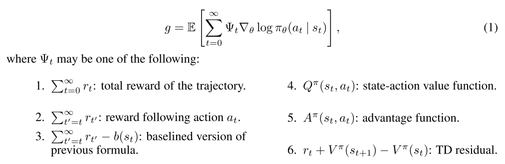
The latter formulas use the definition
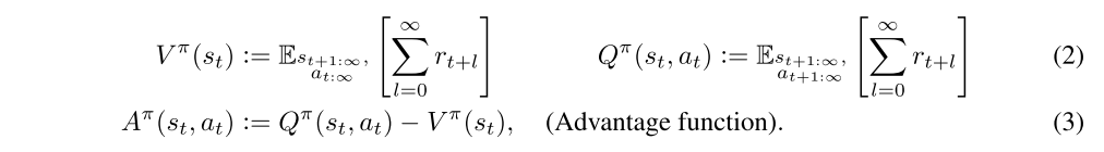
The choice Ψt = Aπ(st, at) yields almost the lowest possible variance, though in practice, the advantage function is not known and must be estimated. This statement can be intuitively justified by the following interpretation of the policy gradient: that a step in the policy gradient direction should increase the probability of better-than-average actions and decrease the probability of worse-than-average actions. The advantage function, by it’s definition Aπ(s, a) = Qπ(s, a) −Vπ(s), measures whether or not the action is better or worse than the policy’s default behavior. Hence, we should choose Ψt to be the advantage function Aπ(st, at), so that the gradient term Ψt∇θ log πθ(at | st) points in the direction of increased πθ(at | st) if and only if Aπ(st, at) > 0.
We will introduce a parameter γ that allows us to reduce variance by downweighting rewards corresponding to delayed effects, at the cost of introducing bias. This parameter corresponds to the discount factor used in discounted formulations of MDPs, but we treat it as a variance reduction parameter in an undiscounted problem. The discounted value functions are given by:
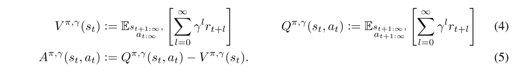
The discounted approximation to the policy gradient is defined as follows:
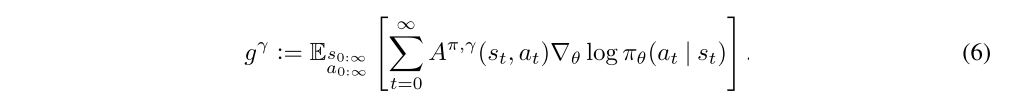
The following section discusses how to obtain biased (but not too biased) estimators for Aπ,γ, giving us noisy estimates of the discounted policy gradient in Equation (6).
Before proceeding, we will introduce the notion of a γ-just estimator of the advantage function, which is an estimator that does not introduce bias when we use it in place of Aπ,γ (which is not known and must be estimated) in Equation (6) to estimate gγ. Consider an advantage estimator Aˆt(s0:∞, a0:∞), which may in general be a function of the entire trajectory
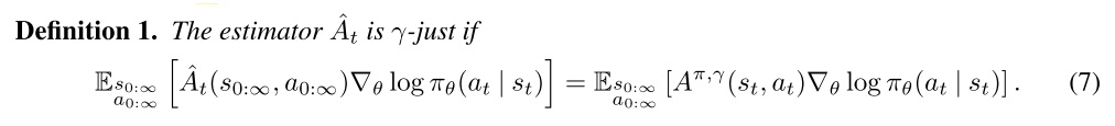
It follows immediately that if ˆAt is γ-just for all t, then
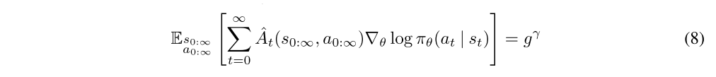
One sufficient condition for Aˆt to be γ-just is that Aˆt decomposes as the difference between two functions Qt and bt, where Qt can depend on any trajectory variables but gives an unbiased estimator of the γ-discounted Q-function, and bt is an arbitrary function of the states and actions sampled before at.
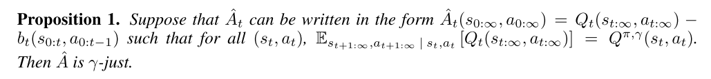
The proof is provided in Appendix B. It is easy to verify that the following expressions are γ-just advantage estimators for Aˆt:

3 Advantage Function Estimation
This section will be concerned with producing an accurate estimate Aˆt of the discounted advantage function Aπ,γ(st, at), which will then be used to construct a policy gradient estimator of the following form:
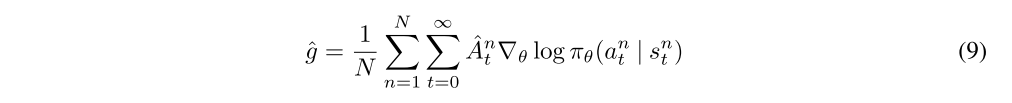
where n indexes over a batch of episodes.
Let V be an approximate value function. Define

i.e., the TD residual of V with discount γ. Note that this can be considered as an estimate of the advantage of the action at. In fact, if we have the correct value function V = Vπ,γ, then it is a γ-just advantage estimator, and in fact, an unbiased estimator of Aπ,γ:
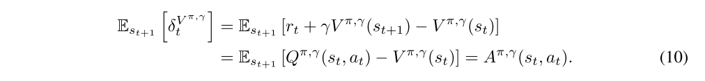
However, this estimator is only γ-just for V = Vπ,γ, otherwise it will yield biased policy gradient estimates.
Next, let us consider taking the sum of k of these δ terms, which we will denote by Atˆ(k):
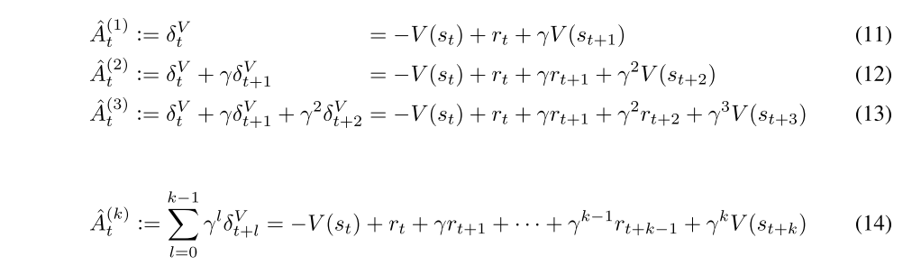
These equations result from a telescoping sum, and we see that Aˆ(k)t involves a k-step estimate of the returns, minus a baseline term −V(st). Analogously to the case of δVt = ˆA(1)t , we can consider Aˆ(k) t to be an estimator of the advantage function, which is only γ-just when V = Vπ,γ. However, note that the bias generally becomes smaller as k → ∞, since the term γkV(st+k) becomes more heavily discounted, and the term −V(st) does not affect the bias. Taking k →∞, we get

which is simply the empirical returns minus the value function baseline.
The GAE(γ, λ) is defined as the exponentially-weighted average of these k-step estimators:
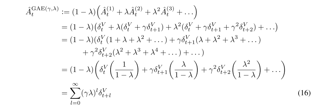
From Equation (16), we see that the advantage estimator has a remarkably simple formula involving a discounted sum of Bellman residual terms. Section 4 discusses an interpretation of this formula as the returns in an MDP with a modified reward function. The construction we used above is closely analogous to the one used to define TD(λ), however TD(λ) is an estimator of the value function, whereas here we are estimating the advantage function.
There are two notable special cases of this formula, obtained by setting λ = 0 and λ = 1.

GAE(γ, 1) is γ-just regardless of the accuracy of V, but it has high variance due to the sum of terms. GAE(γ, 0) is γ-just for V = Vπ,γ and otherwise induces bias, but it typically has much lower variance. The GAE for 0 < λ < 1 makes a compromise between bias and variance, controlled by parameter λ.
We’ve described an advantage estimator with two separate parameters γ and λ, both of which contribute to the bias-variance tradeoff when using an approximate value function. However, they serve different purposes and work best with different ranges of values. γ most importantly determines the scale of the value function Vπ,γ, which does not depend on λ. Taking γ < 1 introduces bias into the policy gradient estimate, regardless of the value function’s accuracy. On the other hand, λ < 1 introduces bias only when the value function is inaccurate. Empirically, we find that the best value of λ is much lower than the best value of γ, likely because λ introduces far less bias than γ for a reasonably accurate value function.
Using the GAE, we can construct a biased estimator of gγ, the discounted policy gradient from Equation (6):
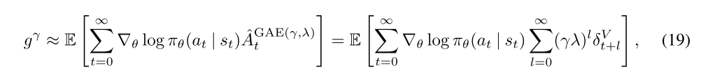
where equality holds when λ = 1.
4 Interpretation as Reward Shaping
In this section, we discuss how one can interpret λ as an extra discount factor applied after performing a reward shaping transformation on the MDP. We also introduce the notion of a response function to help understand the bias introduced by γ and λ.
Reward shaping (paper) refers to the following transformation of the reward function of an MDP: let Φ : S → R be an arbitrary scalar-valued function on state space, and define the transformed reward function by

which in turn defines a transformed MDP. This transformation leaves the discounted advantage function Aπ,γ unchanged for any policy π. To see this, consider the discounted sum of rewards of a trajectory starting with state st:
Value and advantage functions of the transformed MDP,
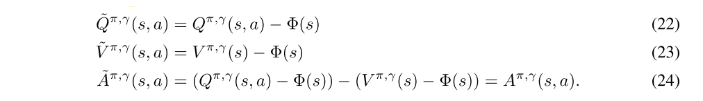
Note that if Φ happens to be the state-value function Vπ,γ from the original MDP, then the transformed MDP has the interesting property that ˜Vπ,γ(s) is zero at every state.
Note that the reward shaping paper showed that the reward shaping transformation leaves the policy gradient and optimal policy unchanged when our objective is to maximize the discounted sum of rewards

In contrast, this paper is concerned with maximizing the undiscounted sum of rewards, where the discount γ is used as a variance-reduction parameter.
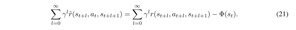
Having reviewed the idea of reward shaping, let us consider how we could use it to get a policy gradient estimate. The most natural approach is to construct policy gradient estimators that use discounted sums of shaped rewards ˜r. However, Equation (21) shows that we obtain the discounted sum of the original MDP’s rewards r minus a baseline term. Next, let’s consider using a “steeper”(更急剧)discount γλ, where 0 ≤ λ ≤ 1. It’s easy to see that the shaped reward ˜r equals the Bellman residual term δV, introduced in Section 3, where we set Φ = V. Letting Φ = V, we see that

Hence, by considering the γλ-discounted sum of shaped rewards, we exactly obtain the GAE from Section 3. As shown previously, λ = 1 gives an unbiased estimate of gγ, whereas λ < 1 gives a biased estimate.
5 Value Function Estimation
A variety of different methods can be used to estimate the value function. When using a nonlinear function approximator to represent the value function, the simplest approach is to solve a nonlinear regression problem:

where

is the discounted sum of rewards, and n indexes over all timesteps in a batch of trajectories. This is sometimes called the Monte Carlo or TD(1) approach for estimating the value function.
For the experiments in this work, we used a trust region method to optimize the value function in each iteration of a batch optimization procedure. The trust region helps us to avoid overfitting to the most recent batch of data. To formulate the trust region problem, we first compute

where φold is the parameter vector before optimization. Then we solve the following constrained optimization problem:

This constraint is equivalent to constraining the average KL divergence between the previous value function and the new value function to be smaller than ε, where the value function is taken to parameterize a conditional Gaussian distribution with mean Vφ(s) and variance σ2.
We compute an approximate solution to the trust region problem using the conjugate gradient algorithm. Specifically, we are solving the quadratic program

where g is the gradient of the objective, and

Note that H is the “Gauss-Newton” approximation of the Hessian of the objective, and it is (up to a σ2 factor) the Fisher information matrix when interpreting the value function as a conditional probability distribution. Using matrix-vector products v → Hv to implement the conjugate gradient algorithm, we compute a step direction

Then we rescale s → αs such that

and take φ = φold + αs. This procedure is analogous to the procedure we use for updating the policy.
6 Experiments
6.1 Policy Optimization Algorithm
While GAE can be used along with a variety of different policy gradient methods, for these experiments, we performed the policy updates using TRPO. TRPO updates the policy by approximately solving the following constrained optimization problem each iteration:
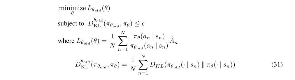
As described in the paper, we approximately solve this problem by linearizing the objective and quadraticizing the constraint, which yields a step in the direction
where F is the average Fisher information matrix, and g is a policy gradient estimate. This policy update yields the same step direction as the natural policy gradient and natural actor-critic, however it uses a different stepsize determination scheme and numerical procedure for computing the step.
Since prior work compared TRPO to a variety of different policy optimization algorithms, we will not repeat these comparisons; rather, we will focus on varying the γ, λ parameters of policy gradient estimator while keeping the underlying algorithm fixed.
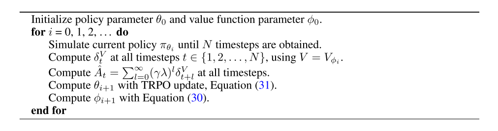
For completeness, the whole algorithm for iteratively updating policy and value function is given below: