Paper 38: Recurrent Models of Visual Attention (RAM)
Abstract
-
Applying CNNs to large images is computationally expensive because the amount of computation scales linearly with the number of image pixels.
-
We present a novel RNN model that is capable of extracting information from an image or video by adaptively selecting a sequence of regions or locations and only processing the selected regions at high resolution.
-
Like CNNs, the proposed model has a degree of translation invariance built-in, but the amount of computation it performs can be controlled independently of the input image size. While the model is non-differentiable, it can be trained using RL methods to learn task-specific policies.
1 Introduction
One important property of human perception is that one does not tend to process a whole scene in its entirety at once. Instead humans focus attention selectively on parts of the visual space to acquire information when and where it is needed, and combine information from different fixations over time to build up an internal representation of the scene, guiding future eye movements and decision making.
In this paper we develop a novel framework for attention-based task-driven visual processing with neural networks. Our model considers attention-based processing of a visual scene as a control problem and is general enough to be applied to static images, videos, or as a perceptual module of an agent that interacts with a dynamic visual environment (e.g. robots, computer game playing agents).
The model is a RNN which processes inputs sequentially, attending to different locations within the images (or video frames) one at a time, and incrementally combines information from these fixations to build up a dynamic internal representation of the scene or environment. Instead of processing an entire image or even bounding box at once, at each step, the model selects the next location to attend to based on past information and the demands of the task. Both the number of parameters in our model and the amount of computation it performs can be controlled independently of the size of the input image, which is in contrast to CNNs whose computational demands scale linearly with the number of image pixels. We describe an end-to-end optimization procedure that allows the model to be trained directly with respect to a given task and to maximize a performance measure which may depend on the entire sequence of decisions made by the model. This procedure uses backpropagation to train the neural-network components and policy gradient to address the non-differentiabilities due to the control problem.
We show that our model can learn effective task-specific strategies for where to look on several image classification tasks as well as a dynamic visual control problem. Our results also suggest that an attention-based model may be better than a CNN at both dealing with clutter and scaling up to large input images.
3 The Recurrent Attention Model (RAM)
In this paper we consider the attention problem as the sequential decision process of a goal-directed agent interacting with a visual environment. At each point in time, the agent observes the environment only via a bandwidth-limited sensor, i.e. it never senses the environment in full. It may extract information only in a local region or in a narrow frequency band. The agent can, however, actively control how to deploy its sensor resources (e.g. choose the sensor location). The agent can also affect the true state of the environment by executing actions. Since the environment is only partially observed the agent needs to integrate information over time in order to determine how to act and how to deploy its sensor most effectively. At each step, the agent receives a scalar reward (which depends on the actions the agent has executed and can be delayed), and the goal of the agent is to maximize the total sum of such rewards.
This formulation encompasses tasks as diverse as object detection in static images and control problems like playing a computer game from the image stream visible on the screen. For a game, the environment state would be the true state of the game engine and the agent’s sensor would operate on the video frame shown on the screen. (Note that for most games, a single frame would not fully specify the game state). The environment actions here would correspond to joystick controls, and the reward would reflect points scored. For object detection in static images the state of the environment would be fixed and correspond to the true contents of the image. The environmental action would correspond to the classification decision (which may be executed only after a fixed number of fixations), and the reward would reflect if the decision is correct.
3.1 Model
The agent is built around a RNN as shown in Figure 1. At each time step, it processes the sensor data, integrates information over time, and chooses how to act and how to deploy its sensor at next time step:
-
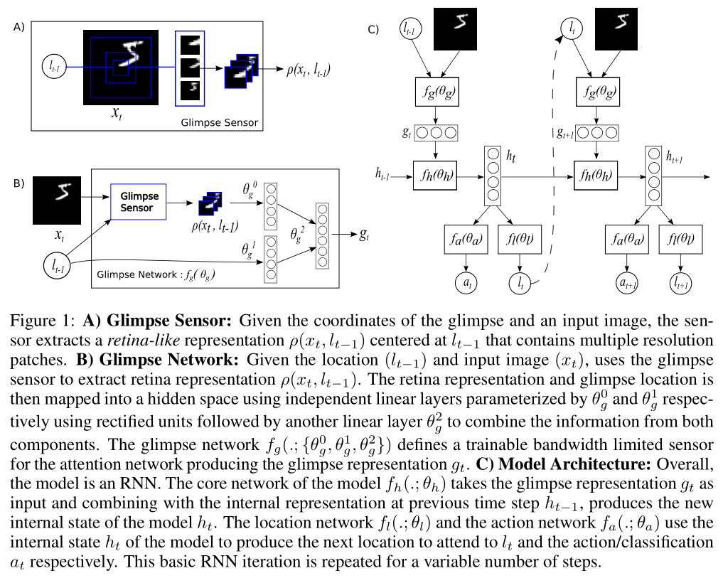
Sensor: At each step t the agent receives a (partial) observation of the environment in the form of an image xt. The agent does not have full access to this image but rather can extract information from xt via its bandwidth limited sensor ρ, e.g. by focusing the sensor on some region or frequency band of interest.In this paper we assume that the bandwidth-limited sensor extracts a retina-like representation ρ(xt, lt−1) around location lt−1 from image xt. It encodes the region around l at a high-resolution but uses a progressively lower resolution for pixels further from l, resulting in a vector of much lower dimensionality than the original image x. We will refer to this low-resolution representation as a glimpse. The glimpse sensor is used inside what we call the glimpse network fg to produce the glimpse feature vector gt = fg(xt, lt−1; θg) where θg = {θ0g, θ1g, θ2g} (Figure 1 B).
-
Internal state: The agent maintains an internal state which summarizes information extracted from the history of past observations; it encodes the agent’s knowledge of the environment and is instrumental(有用的)to deciding how to act and where to deploy the sensor. This internal state is formed by the hidden units ht of the RNN and updated over time by the core network: ht = fh(ht−1, gt; θh). The external input to the network is the glimpse feature vector gt. -
Actions: At each step, the agent performs two actions: it decides how to deploy its sensor via the sensor control lt, and an environment action at which might affect the state of the environment. The nature of the environment action depends on the task. In this work, the location actions are chosen stochastically from a distribution parameterized by the location network fl(ht; θl) at time t: lt ∼ p(·|fl(ht; θl)). The environment action at is similarly drawn from a distribution conditioned on a second network output at ∼ p(·|fa(ht; θa)). For classification it is formulated using a softmax output and for dynamic environments, its exact formulation depends on the action set defined for that particular environment (e.g. joystick movements, motor control, …). Finally, our model can also be augmented with an additional action that decides when it will stop taking glimpses. This could, for example, be used to learn a cost-sensitive classifier by giving the agent a negative reward for each glimpse it takes, forcing it to trade off making correct classifications with the cost of taking more glimpses. -
Reward: After executing an action the agent receives a new visual observation of the environment xt+1 and a reward signal rt+1. The goal of the agent is to maximize the sum of the reward signal which is usually very sparse and delayed:
In the case of object recognition, for example, rT = 1 if the object is classified correctly after T steps and 0 otherwise.
The above setup is a special instance of what is known in the RL community as a POMDP. The true state of the environment (which can be static or dynamic) is unobserved. In this view, the agent needs to learn a (stochastic) policy π((lt, at)|s1:t; θ) with parameters θ that, at each step t, maps the history of past interactions with the environment s1:t = x1, l1, a1, . . . xt−1, lt−1, at−1, xt to a distribution over actions for the current time step, subject to the constraint of the sensor. In our case, the policy π is defined by the RNN outlined above, and the history st is summarized in the state of the hidden units ht. We will describe the specific choices for the above components in Section 4.
3.2 Training
The parameters of our agent are given by the parameters of the glimpse network, the core network (Figure 1 C), and the action network θ = {θg, θh, θa} and we learn these to maximize the total reward the agent can expect when interacting with the environment.
Viewing the problem as a POMDP, allows us to bring techniques from the RL literature to bear: a sample approximation to the gradient is given by

Variance Reduction: Equation (1) provides us with an unbiased estimate of the gradient but it may have high variance. It is therefore common to consider a gradient estimate of the form

Using a Hybrid Supervised Loss: The algorithm described above allows us to train the agent when the “best” actions are unknown, and the learning signal is only provided via the reward. For instance, we may not know a priori which sequence of fixations provides most information about an unknown image, but the total reward at the end of an episode will give us an indication whether the tried sequence was good or bad.
However, in some situations we do know the correct action to take: For instance, in an object detection task the agent has to output the label of the object as the final action. For the training images this label will be known and we can directly optimize the policy to output the correct label associated with a training image at the end of an observation sequence. This can be achieved, as is common in supervised learning, by maximizing the conditional probability of the true label given the observations from the image, i.e. by maximizing
