Paper 39: Deep Attention Recurrent Q-Network (DARQN)
Abstract
-
We present an extension of DQN by “soft” and “hard” attention mechanisms.
-
Tests of the proposed Deep Attention Recurrent Q-Network (DARQN) algorithm on multiple Atari 2600 games show level of performance superior to that of DQN.
-
Built-in attention mechanisms allow a direct online monitoring of the training process by highlighting the regions of the game screen the agent is focusing on when making decisions.
1 Introduction and Related Work
DQN decides on the next optimal action based on the visual information corresponding to the last four game states encountered by the agent. Therefore, the algorithm cannot master those games that require a player to remember events more distant than four screens in the past. It is for this reason that the Deep Recurrent Q-Network (DRQN) was proposed, a combination of LSTM and DQN in which (i) the fully connected layer in the latter is replaced for a LSTM one, and (ii) only the last visual frame at each timestep is used as DQN’s input. The authors report that despite seeing only one visual frame, DRQN is still capable integrating relevant information across the frames. Nonetheless, no systematic improvement in Atari game scores over the results was observed.
Another drawback of DQN is its long training time, which is a critical component to the researchers’ ability to carry out experiments with different network architectures and algorithm’s parameter settings. A new massively parallel version of DQN was proposed to address this problem. The authors report that its performance surpassed non-distributed DQN in 41 of the 49 games. However, extensive parallelization is not the only and, probably, not the most efficient remedy to the problem.
Recent achievements of visual attention models in caption generation, object tracking, and machine translation have induced the authors of this paper to conduct a series of experiments so as to assess possible benefits from incorporating attention mechanisms into the structure of the DRQN algorithm. The main advantage of utilizing these mechanisms is that DRQN acquires the ability to select and then focus on relatively small informative regions of an input image, thus helping to reduce the total number of parameters in the DNN and computational operations needed for training and testing it. In contrast to DRQN, in this case, LSTM layer stores the data used not only for making decision on the next action, but also for choosing the next region of attention. In addition to computational speedups, attention-based models can also add some degree of interpretability to the Deep Q-Learning process by providing researchers with an opportunity to visualize “where” and “what” the agent’s attention is focusing on.
2 Deep Attention Recurrent Q-Network
The Deep Attention Recurrent Q-Network
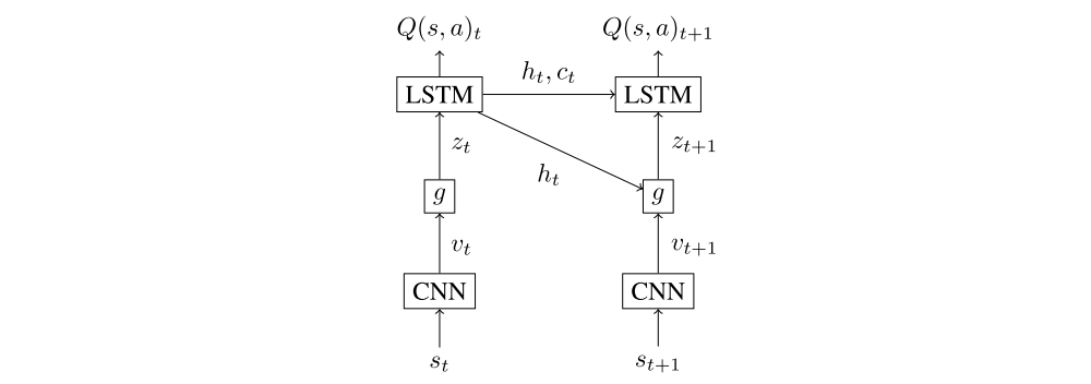
The DARQN architecture is schematically shown in the figure above and consists of three types of networks: convolutional (CNN), attention, and recurrent. At each time step t, CNN receives a representation of the current game state st in the form of a visual frame, based on which it produces a set of D feature maps, each having a dimension of m×m. The attention network transforms these maps into a set of vectors

L = m ∗ m and outputs their linear combination zt, called a context vector. The recurrent network, in our case LSTM, takes as input the context vector, along with the previous hidden state ht−1 and memory state ct−1, and produces hidden state ht that is used by (i) a linear layer for evaluating Q-value of each action at that the agent can take being in state st, (ii) the attention network for generating a context vector at the next time step t + 1. In the following subsections, we consider two approaches to the context vector calculation. As will be shown, they have important differences in the training procedure.
2.1 Soft attention
The “soft” attention mechanism assumes that the context vector can be represented as a weighted sum of all vectors, each of which corresponds to the features extracted by CNN at different image regions. Weights in this sum are chosen in proportion to the vectors relative importance assessed by the attention network g. The network contains two fully connected layers followed by a softmax activation. Its output may be written as:

where Z is a normalizing constant, W is a weights matrix, Linear(x) = Ax + b is an affine(仿射)transformation with some weights matrix A and bias b. Once we have defined the importance of each location vector, we can calculate the context vector zt:

Other networks depicted in Figure 1 have a standard form, the details of their realization are discussed in Section 3. The whole DARQN model is trained by minimizing a sequence of loss functions:

where

is an approximate target value, The capital ε is an environment distribution, ρ(st, at) is a behaviour distribution selected as ε-greedy strategy, θt is a vector of all DARQN weights, including those belonging to the attention network. To optimize the loss function, we use the standard Q-learning update rule:

All functions in DARQN are differentiable; therefore, the gradient exists for each parameter, and the whole model can be trained end-to-end. The suggested algorithm also utilizes two training techniques, target network and experience replay.
2.2 Hard attention
The “hard” attention mechanism requires sampling only one attention location from L available at each time step t in accordance with some stochastic attention policy πg. In our case, this policy is represented by the neural network g whose output consists of location selection probabilities and whose weights are the policy parameters. In order to train a network with stochastic units, the statistical gradient-following algorithm REINFORCE may be used. There are several successful examples of integrating this algorithm with DL. The suggested algorithm is trained by minimizing a sequence of loss functions. Assume that st (and therefore vt) was sampled from the environment distribution affected by the attention policy πg(it | vt, ht−1), a categorical distribution with parameters given by a softmax layer of the attention network g. Then, in the policy gradient approach, updates of the policy parameters may be written as:

where Rt is a future discounted return after the agent selects the attention location it. In order to approximate this value, a separate neural network Gt = Linear(ht) has been introduced. This network is trained by regressing towards the expected value of Yt. The final update rule for the attention network’s parameters has the following form:
