Paper 40: Show, Attend and Tell: Neural Image Caption Generation with Visual Attention
Abstract
-
We introduce an attention based model that automatically learns to describe the content of images.
-
We describe how we can train this model in a deterministic manner using standard backpropagation techniques and stochastically by maximizing a variational lower bound.
-
We also show through visualization how the model is able to automatically learn to fix its gaze on salient objects while generating the corresponding words in the output sequence.
1 Introduction
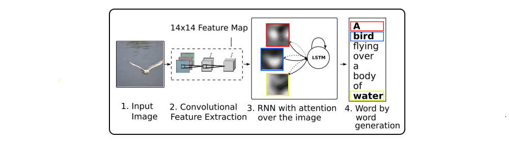
Figure 1
In this paper, we describe approaches to caption generation that attempt to incorporate a form of attention with two variants: a “hard” attention mechanism and a “soft” attention mechanism. We also show how one advantage of including attention is the ability to visualize what the model “sees”. We investigate models that can attend to salient part of an image while generating its caption.
The contributions of this paper are the following:
-
We introduce two attention-based image caption generators under a common framework:
-
a “soft” deterministic attention mechanism trainable by standard back-propagation methods
-
a “hard” stochastic attention mechanism trainable by maximizing an approximate variational lower bound or equivalently by REINFORCE.
-
-
We show how we can gain insight and interpret the results of this framework by visualizing “where” and “what” the attention focused on.
-
Finally, we quantitatively validate the usefulness of attention in caption generation with SOTA performance on three benchmark datasets.
3 Image Caption Generation with Attention Mechanism
3.1. Model Details
In this section, we describe the two variants of our attention-based model by first describing their common framework. The main difference is the definition of the φ function which we describe in detail in Section 4. We denote vectors with bolded font and matrices with capital letters. In our description below, we suppress bias terms for readability.
3.1.1 Encoder: Convolutional Features
Our model takes a single raw image and generates a caption y encoded as a sequence of 1-of-K encoded words.

where K is the size of the vocabulary and C is the length of the caption.
We use a CNN in order to extract a set of feature vectors which we refer to as annotation vectors. The extractor produces L vectors, each of which is a D-dimensional representation corresponding to a part of the image.

In order to obtain a correspondence between the feature vectors and portions of the 2-D image, we extract features from a lower convolutional layer unlike previous work which instead used a fully connected layer. This allows the decoder to selectively focus on certain parts of an image by selecting a subset of all the feature vectors.
3.1.2 Decoder: Long Short-Term Memory Network
We use a LSTM network that produces a caption by generating one word at every time step conditioned on a context vector, the previous hidden state and the previously generated words.
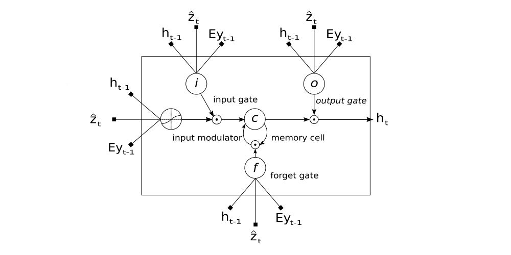
Figure 2
A LSTM cell, lines with bolded squares imply projections with a learnt weight vector. Each cell learns how to weigh its input components (input gate), while learning how to modulate(调节)that contribution to the memory (input modulator). It also learns weights which erase the memory cell (forget gate), and weights which control how this memory should be emitted (output gate).
Using Ts,t to denote a simple affine transformation with parameters that are learned,
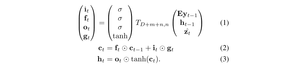
Here, it, ft, ct, ot, ht are the input, forget, memory, output and hidden state of the LSTM, respectively. The vector zˆ (D-dimension) is the context vector, capturing the visual information associated with a particular input location, as explained below. E (m×K-dimension) is an embedding matrix. Let m and n denote the embedding and LSTM dimensionality respectively and σ and ⊙ be the logistic sigmoid activation and element-wise multiplication respectively.
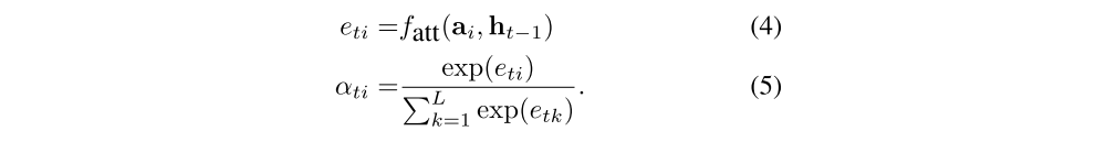
In simple terms, the context vector zˆt (equations (1)–(3)) is a dynamic representation of the relevant part of the image input at time t. We define a mechanism φ that computes zˆt from the annotation vectors ai, i = 1, . . . , L corresponding to the features extracted at different image locations. For each location i, the mechanism generates a positive weight αi which can be interpreted either as the probability that location i is the right place to focus for producing the next word (the “hard” but stochastic attention mechanism), or as the relative importance to give to location i in blending the ai’s together. The weight αi of each annotation vector ai is computed by an attention model fatt for which we use a multilayer perceptron conditioned on the previous hidden state ht−1. For emphasis, we note that the hidden state varies as the output RNN advances in its output sequence: “where” the network looks next depends on the sequence of words that has already been generated.
Once the weights (which sum to one) are computed, the context vector zˆt is computed by

where φ is a function that returns a single vector given the set of annotation vectors and their corresponding weights. The details of φ function are discussed in Sec. 4.
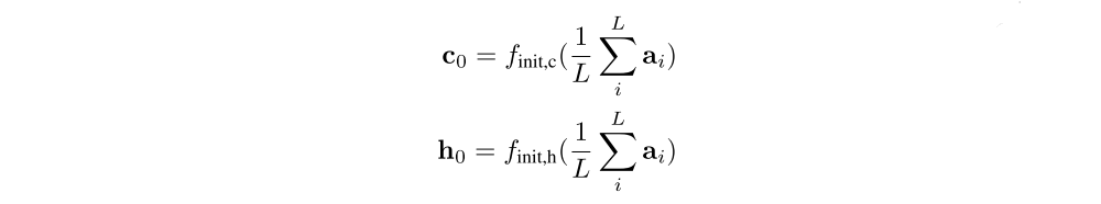
The initial memory state and hidden state of the LSTM are predicted by an average of the annotation vectors fed through two separate MLPs (init,c and init,h):
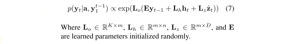
In this work, we use a deep output layer to compute the output word probability given the LSTM state, the context vector and the previous word:
4 Learning Stochastic “Hard” vs Deterministic “Soft” Attention
In this section we discuss two alternative mechanisms for the attention model fatt: stochastic attention and deterministic attention.
4.1 Stochastic “Hard” Attention
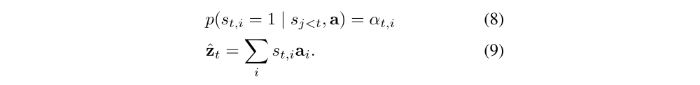
We represent the location variable st as where the model decides to focus attention when generating the t-th word. st,i is an indicator one-hot variable which is set to 1 if the i-th location (out of L) is the one used to extract visual features. By treating the attention locations as intermediate latent variables, we can assign a multinoulli distribution parametrized by {αi}, and view zˆt as a random variable:
We define a new objective function Ls that is a variational lower bound on the marginal log-likelihood log p(y | a) of observing the sequence of words y given image features a. The learning algorithm for the parameters W of the models can be derived by directly optimizing Ls:
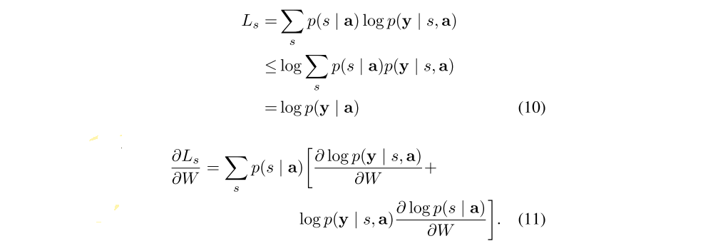
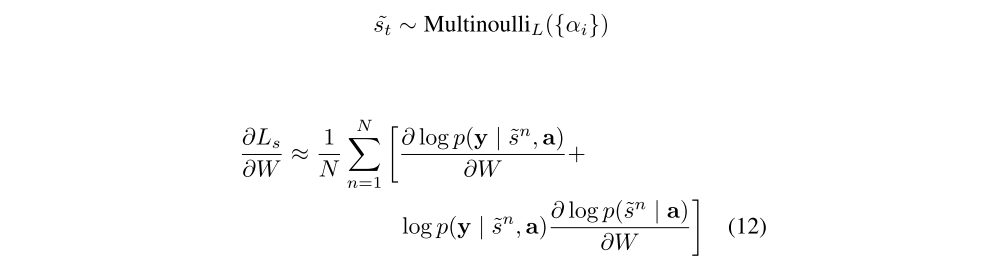
Equation 11 suggests a Monte Carlo based sampling approximation of the gradient with respect to the model parameters. This can be done by sampling the location st from a multinouilli distribution defined by Equation 8.
A moving average baseline is used to reduce the variance in the Monte Carlo estimator of the gradient. Upon seeing the k-th mini-batch, the moving average baseline is estimated as an accumulated sum of the previous log likelihoods with exponential decay:

To further reduce the estimator variance, an entropy term on the multinouilli distribution H[s] is added. Also, with probability 0.5 for a given image, we set the sampled attention location ˜s to its expected value α. Both techniques improve the robustness of the stochastic attention learning algorithm. The final learning rule for the model is then the following:
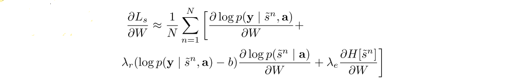
where, λr and λe are two hyper-parameters set by cross-validation.
In making a hard choice at every point, φ({ai}, {αi}) from Equation 6 is a function that returns a sampled ai at every point in time based upon a multinouilli distribution parameterized by α.
4.2 Deterministic “Soft” Attention
Learning stochastic attention requires sampling the attention location st each time, instead we can take the expectation of the context vector zˆt directly,

and formulate a deterministic attention model by computing a soft attention weighted annotation vector

This corresponds to feeding in a soft α weighted context into the system. The whole model is smooth and differentiable under the deterministic attention, so learning end-to-end is trivial by using standard backpropagation.
Learning the deterministic attention can also be understood as approximately optimizing the marginal likelihood in Equation 10 under the attention location random variable st from Sec. 4.1. The hidden activation of LSTM ht is a linear projection of the stochastic context vector zˆt followed by tanh non-linearity. To the first order Taylor approximation, the expected value Ep(st|a)[ht] is equal to computing ht using a single forward prop with the expected context vector Ep(st|a)[zˆt]. Considering Eq. 7, let

nt,i (we can view it as logit) denotes nt computed by setting the random variable zˆ value to ai. We define the normalized weighted geometric mean for the softmax k-th word prediction:
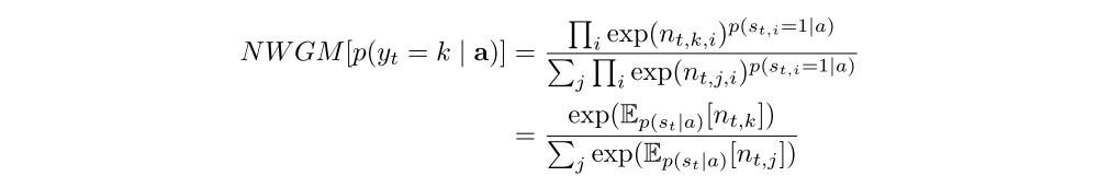
The equation above shows the normalized weighted geometric mean of the caption prediction can be approximated well by using the expected context vector, where

It shows that the NWGM of a softmax unit is obtained by applying softmax to the expectations of the underlying linear projections. Also, from the results in previous paper, NWGM[p(yt = k | a)] ≈ E[p(yt = k | a)] under softmax activation. That means the expectation of the outputs over all possible attention locations induced by random variable st is computed by simple feedforward propagation with expected context vector E[zˆt]. In other words, the deterministic attention model is an approximation to the marginal likelihood over the attention locations.
4.2.1 Doubly Stochastic Attention
By construction,

as they are the output of a softmax. In training the deterministic version of our model we introduce a form of doubly stochastic regularization, where we also encourage

This can be interpreted as encouraging the model to pay equal attention to every part of the image over the course of generation. In our experiments, we observed that this penalty was important quantitatively to improving overall BLEU score and that qualitatively this leads to more rich and descriptive captions. In addition, the soft attention model predicts a gating scalar β from previous hidden state ht−1 at each time step t, such that,

where

We notice our attention weights put more emphasis on the objects in the images by including the the scalar β.
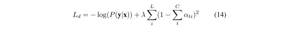
Concretely, the model is trained end-to-end by minimizing the following penalized negative log-likelihood: