Paper 44: Noisy Networks for Exploration (Noisy DQN)
Abstract
-
We introduce NoisyNet, a DRL agent with parametric noise added to its weights, and show that the induced stochasticity of the agent’s policy can be used to aid efficient exploration.
-
The parameters of the noise are learned with gradient descent along with the remaining network weights. NoisyNet is straightforward to implement and adds little computational overhead.
-
We find that replacing the conventional exploration heuristics for A3C, DQN and Dueling agents (entropy reward and ε-greedy respectively) with NoisyNet yields substantially higher scores for a wide range of Atari games, in some cases advancing the agent from sub to super-human performance.
1 Introduction
Despite the wealth of research into efficient methods for exploration in RL, most exploration heuristics rely on random perturbations(扰动)of the agent’s policy, such as ε-greedy or entropy regularization, to induce novel behaviours. However such local ‘dithering’ perturbations are unlikely to lead to the large-scale behavioural patterns needed for efficient exploration in many environments.
Optimism in the face of uncertainty is a common exploration heuristic in RL. Various forms of this heuristic often come with theoretical guarantees on agent performance. However, these methods are often limited to small state-action spaces or to linear function approximations and are not easily applied with more complicated function approximators such as neural networks.
A more structured approach to exploration is to augment the environment’s reward signal with an additional intrinsic motivation term that explicitly rewards novel discoveries. Many such terms have been proposed, including learning progress, compression progress, variational information maximization and prediction gain. One problem is that these methods separate the mechanism of generalization from that of exploration; the metric for intrinsic reward, and its weighting relative to the environment reward, must be chosen by the experimenter, rather than learned from interaction with the environment. Without due care, the optimal policy can be altered or even completely obscured by the intrinsic rewards; furthermore, dithering perturbations are usually needed as well as intrinsic reward to ensure robust exploration. Exploration in the policy space itself, for example, with evolutionary or black box algorithms, usually requires many prolonged interactions with the environment. Although these algorithms are quite generic and can apply to any type of parametric policies (including neural networks), they are usually not data efficient and require a simulator to allow many policy evaluations.
We propose a simple alternative approach, called NoisyNet, where learned perturbations of the network weights are used to drive exploration. The key insight is that a single change to the weight vector can induce a consistent, and potentially very complex, state-dependent change in policy over multiple time steps – unlike dithering approaches where decorrelated (and, in the case of ε-greedy, state-independent) noise is added to the policy at every step. The perturbations are sampled from a noise distribution. The variance of the perturbation is a parameter that can be considered as the energy of the injected noise. These variance parameters are learned using gradients from the RL loss function, along side the other parameters of the agent. The approach differs from parameter compression schemes such as variational inference and flat minima search since we do not maintain an explicit distribution over weights during training but simply inject noise in the parameters and tune its intensity automatically. Consequently, it also differs from Thompson sampling as the distribution on the parameters of our agents does not necessarily converge to an approximation of a posterior distribution.
At a high level our algorithm is a randomized value function, where the functional form is a neural network. Randomized value functions provide a provably efficient means of exploration. Previous attempts to extend this approach to DNNs required many duplicates of sections of the network. By contrast in our NoisyNet approach while the number of parameters in the linear layers of the network is doubled, as the weights are a simple affine transform of the noise, the computational complexity is typically still dominated by the weight by activation multiplications, rather than the cost of generating the weights. Additionally, it also applies to policy gradient methods such as A3C out of the box. Most recently someone presented a similar technique where constant Gaussian noise is added to the parameters of the network. Our method thus differs by the ability of the network to adapt the noise injection with time and it is not restricted to Gaussian noise distributions. We need to emphasis that the idea of injecting noise to improve the optimization process has been thoroughly studied in the literature of supervised learning and optimization under different names and graduated optimization. These methods often rely on a noise of vanishing size that is non-trainable, as opposed to NoisyNet which tunes the amount of noise by gradient descent.
NoisyNet can also be adapted to any DRL algorithm and we demonstrate this versatility by providing NoisyNet versions of DQN2015, Dueling and A3C algorithms. Experiments on 57 Atari games show that NoisyNet-DQN and NoisyNet-Dueling achieve striking gains when compared to the baseline algorithms without significant extra computational cost, and with less hyper parameters to tune. Also the noisy version of A3C provides some improvement over the baseline.
2 Background
2.1 Markov Decision Processes and Reinforcement Learning
2.2 Deep Reinforcement Learning
3 NoisyNets for Reinforcement Learning
NoisyNets are neural networks whose weights and biases are perturbed by a parametric function of the noise. These parameters are adapted with gradient descent. More precisely, let y = fθ(x) be a neural network parameterized by the vector of noisy parameters θ which takes the input x and outputs y. We represent the noisy parameters θ as

where

is a set of vectors of learnable parameters, ε is a vector of zero-mean noise with fixed statistics and ⊙ represents element-wise multiplication. The usual loss of the neural network is wrapped by expectation over the noise ε:

Optimization now occurs with respect to the set of parameters ζ.
即计算梯度的时候只计算涉及 ξ 中的参数,因为 ε 是噪声;计算损失的时候仍然按照以前的方法,把 θ 当作参数参加运算。
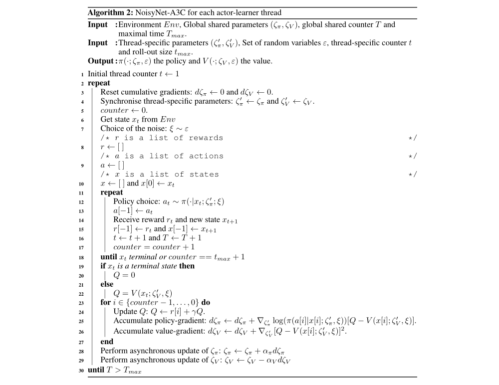
Consider a linear layer of a neural network with p inputs and q outputs, represented by

where x (p-dimension) is the layer input, w (q×p-dimension) the weight matrix, and b (q-dimension) the bias. The corresponding noisy linear layer is defined as:

The parameters µw (q×p-dimension), µb (q-dimension), σw (q×p-dimension) and σb (q-dimension) are learnable whereas εw (q×p-dimension) and εb (q-dimension) are noise random variables (the specific choices of this distribution are described below). We provide a graphical representation of a noisy linear layer in Figure 1.
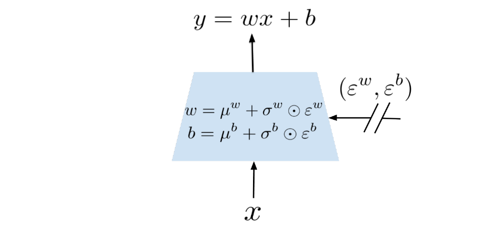
Figure 1: Graphical representation of a noisy linear layer.
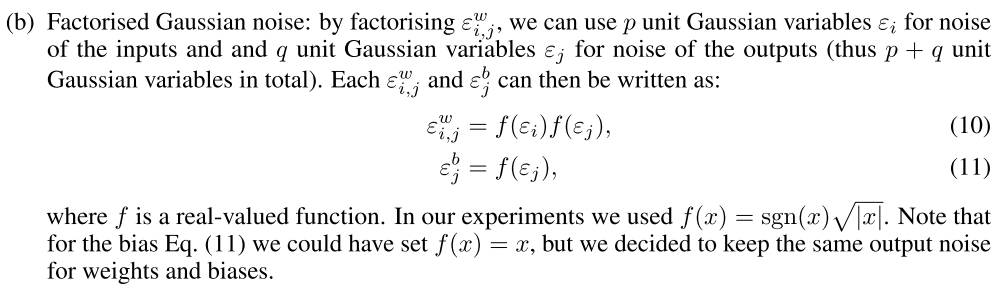
We now turn to explicit instances of the noise distributions for linear layers in a noisy network. We explore two options: Independent Gaussian noise, which uses an independent Gaussian noise entry per weight and Factorized Gaussian noise, which uses an independent noise per each output and another independent noise per each input. The main reason to use factorized Gaussian noise is to reduce the compute time of random number generation in our algorithms. This computational overhead is especially prohibitive in the case of single-thread agents such as DQN and Duelling. For this reason we use factorized noise for DQN and Duelling and independent noise for the distributed A3C, for which the compute time is not a major concern.
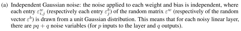
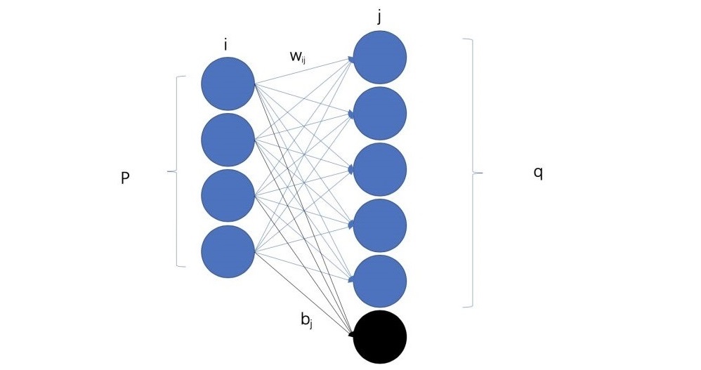
Figure 2: Two layers of a neural network.
Since the loss of a noisy network,

is an expectation over the noise, the gradients are straightforward to obtain:

We use a Monte Carlo approximation to the above gradients, taking a single sample ξ at each step of optimization:

3.1 Deep Reinforcement Learning with NoisyNets
We now turn to our application of noisy networks to exploration in DRL. Noise drives exploration in many methods for RL, providing a source of stochasticity external to the agent and the RL task at hand. Either the scale of this noise is manually tuned across a wide range of tasks (as is the practice in general purpose agents such as DQN or A3C) or it can be manually scaled per task. Here we propose automatically tuning the level of noise added to an agent for exploration, using the noisy networks training to drive down (or up) the level of noise injected into the parameters of a neural network, as needed.
A noisy network agent samples a new set of parameters after every step of optimization. Between optimization steps, the agent acts according to a fixed set of parameters (weights and biases). This ensures that the agent always acts according to parameters that are drawn from the current noise distribution.
-
Deep Q-Networks (DQN) and Dueling.
We apply the following modifications to both DQN and Dueling: first, ε-greedy is no longer used, but instead the policy greedily optimizes the (randomized) action-value function. Secondly, the fully connected layers of the value network are parameterized as a noisy network, where the parameters are drawn from the noisy network parameter distribution after every replay step. We used factorized Gaussian noise as explained in (b) from Sec. 3. For replay, the current noisy network parameter sample is held fixed across the batch. Since DQN and Dueling take one step of optimization for every action step, the noisy network parameters are re-sampled before every action. We call the new adaptations of DQN and Dueling, NoisyNet-DQN and NoisyNet-Dueling, respectively.
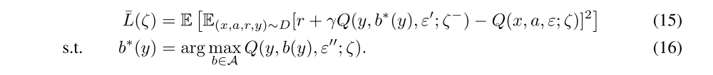
We now provide the details of the loss function that our variant of DQN is minimizing. When replacing the linear layers by noisy layers in the network (respectively in the target network), the parameterized action-value function Q(x, a, ε; ζ) (respectively Q(x, a, ε’; ζ−)) can be seen as a random variable and the DQN loss becomes the NoisyNet-DQN loss:

where the outer expectation is with respect to distribution of the noise variables ε for the noisy value function Q(x, a, ε; ζ) and the noise variable ε’ for the noisy target value function Q(y, b, ε’; ζ−). Computing an unbiased estimate of the loss is straightforward as we only need to compute, for each transition in the replay buffer, one instance of the target network and one instance of the online network. We generate these independent noises to avoid bias due to the correlation between the noise in the target network and the online network. Concerning the action choice, we generate another independent sample ε’’ for the online network and we act greedily with respect to the corresponding output action-value function.
Similarly the loss function for NoisyNet-Dueling is defined as:
-
Asynchronous Advantage Actor Critic (A3C).
A3C is modified in a similar fashion to DQN: firstly, the entropy bonus of the policy loss is removed. Secondly, the fully connected layers of the policy network are parameterized as a noisy network. We used independent Gaussian noise as explained in (a) from Sec. 3. In A3C, there is no explicit exploratory action selection scheme (such as ε-greedy); and the chosen action is always drawn from the current policy. For this reason, an entropy bonus of the policy loss is often added to discourage updates leading to deterministic policies. However, when adding noisy weights to the network, sampling these parameters corresponds to choosing a different current policy which naturally favours exploration. As a consequence of direct exploration in the policy space, the artificial entropy loss on the policy can thus be omitted. New parameters of the policy network are sampled after each step of optimization, and since A3C uses n step returns, optimization occurs every n steps. We call this modification of A3C, NoisyNet-A3C.
Indeed, when replacing the linear layers by noisy linear layers (the parameters of the noisy network are now noted ζ), we obtain the following estimation of the return via a roll-out of size k:

As A3C is an on-policy algorithm the gradients are unbiased when noise of the network is consistent for the whole roll-out. Consistency among action value functions Qˆi is ensured by letting the noise be the same throughout each rollout, i.e., ∀i, εi = ε. Additional details are provided in the Appendix.
3.2 Initialization of Noisy Networks
In the case of an unfactorized noisy networks, the parameters µ and σ are initialized as follows. Each element µi,j is sampled from independent uniform distributions

where p is the number of inputs to the corresponding linear layer, and each element σi,j is simply set to 0.017 for all parameters. This particular initialization was chosen because similar values worked well for the supervised learning tasks described in previous paper, where the initialization of the variances of the posteriors and the variances of the prior are related. We have not tuned for this parameter, but we believe different values on the same scale should provide similar results.
For factorized noisy networks, each element µi,j was initialized by a sample from an independent uniform distributions

and each element σi,j was initialized to a constant σ0/√p . The hyperparameter σ0 is set to 0.5.
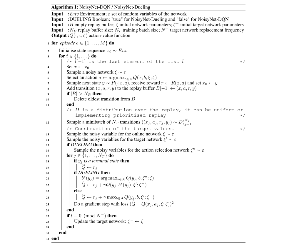
Appendix C Algorithms
C.1 NoisyNet-DQN and NoisyNet-Dueling
C.2 NoisyNet-A3C