Paper 46: A Distributional Perspective on Reinforcement Learning (Categorical DQN)
1 Q-learning
In RL we are interested in maximizing the expected return so we usually work directly with those expectations. For instance, in Q-learning with function approximation we want to minimize the error
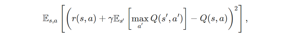
or, equivalently,
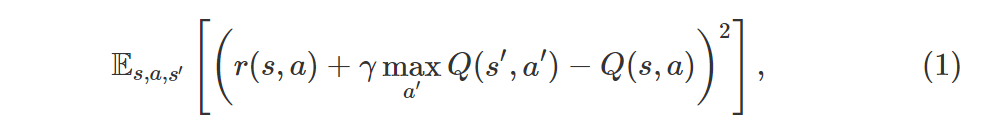
where r(s, a) is the expected immediate reward. In semi-gradient methods we do this by moving Q(s, a) towards the target r(s, a) + γmaxa′Q(s′, a′), pretending that the target is constant, and in DQN2015 we even freeze the “target network” to improve stability even further.
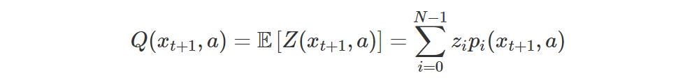
The main idea of Distributional RL is to work directly with the full distribution of the return rather than with its expectation. Let the random variable Z(s, a) be the return obtained by starting from state s, performing action a and then following the current policy. Then

Instead of trying to minimize the error (1), which is basically a distance between expectations, we can instead try to minimize a distributional error, which is a distance between full distributions:
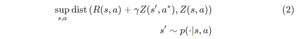
where you can mentally replace sup with max, R(s, a) is the random variable for the immediate reward, and

Note that we’re still using Q(s, a), i.e. the expected return, to decide which action to pick, but we’re trying to optimize distributions rather than expectations (of those distributions).
There’s a subtlety in expression (2): if s, a are constant, Z(s, a) is a random variable, but even more so when s or a are themselves random variables!
2 Policy Evaluation
Let’s consider policy evaluation for a moment. In this case we want to minimize

We can define the Bellman operator for evaluation as follows:

The Bellman operator Tπ is a γ-contraction, meaning that

so, since Qπ is a unique fixed point (i.e. TQ = Q ⟺ Q = Qπ), we must have that T∞Q = Qπ, disregarding approximation errors.
It turns out that this result can be ported to the distributional setting. Let’s define the Bellman distribution operator for evaluation in an analogous way:
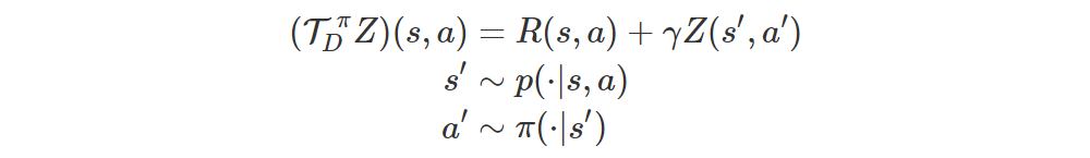
The operator is a γ-contraction in the Wasserstein distance W, i.e.

This isn’t true for the KL divergence.
Unfortunately, this result doesn’t hold for the control (the one with the max) version of the distributional operator.
3 KL divergence
3.1 Definition
I warn you that this subsection is highly informal.
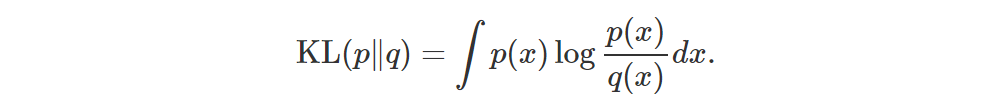
If p and q are two distributions with same support (i.e. their pdfs are non-zero at the same points), then their KL divergence is defined as follows:
Let’s consider the discrete case:
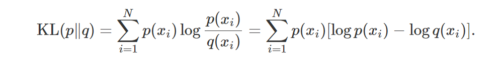
As we can see, we’re basically comparing the scores at the points x1,…,xN, weighting each comparison according to p(xi). Note that the KL doesn’t make use of the values xi directly: only their probabilities are used! Moreover, if p and q have different supports, the KL is undefined.
3.2 How to use it
Now say we’re using DQN and extract (s, a, r, s′) from the replay buffer. A “sample of the target distribution” is r + γ Z(s′, a∗), where a∗ = argmaxa′Q(s′, a′). We want to move Z(s, a) towards this target (by keeping the target fixed).
I called r + γ Z(s′, a∗) a “sample of a distribution”, but the correct way to say it is that r + γ Z(s′, a∗) is a collection of samples of the real target distribution. The target distribution we want to learn is r + γ Z(s′, a∗) where r and s′ are random variables. Since we sampled r and s′, then the atoms of r + γ Z(s′, a∗) are just samples from the real target distribution and not a representation in atom form of that distribution. Indeed, to get a single sample from the real target distribution, we should first sample r and s′, and, finally, sample from the distribution r + γ Z(s′, a∗). This is almost exactly what we’re doing since r and s′ extracted from the replay buffer were indeed sampled. The only difference is that instead of sampling from r + γ Z(s′, a∗), we use all its atoms.
Let’s say we have a net which models Z by taking a state s and returning a distribution Z(s, a) for each action. For instance, we can represent each distribution through a softmax like we often do in deep Learning for classification tasks. In particular, let’s choose some fixed values x1,…,xN for the support of all the distributions returned by the net. To simplify things, let’s make them equidistant so that

The pmf looks like a comb:

Since the values x1,…,xN are fixed, we just have to return N probabilities for each Z(s, a), so the net takes a single state and returns |A|N scalars, where |A| is the number of possible actions.
If p1,…,pN and q1,…,qN are the probabilities of the two distributions p and q, then their KL is simply
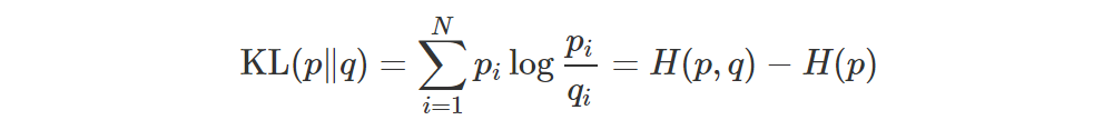
and if you’re optimizing wrt q (i.e. you’re moving q towards p), then you can drop the entropy term.
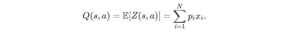
Also, we can recover Q(s, a) very easily:
The interesting part is the transformation. In distributional Q-learning we want to move Z(s, a) towards r + γ Z(s′, a∗), but how do we put p in “standard comb form”? This is the projection part. To form the target distribution we start from p = Z(s′, a∗), which is already in the standard form p1,…,pN and we look at the pairs (x1, p1),…,(xN, pN) as if they represented samples with weights (atoms). This means that we can transform the distribution p just by transforming the position of its atoms. The transformed atoms corresponding to r + γ Z(s′, a∗) are

Note that the weights pi don’t change. The problem is that now we have atoms which aren’t in the standard positions x1,…,xN. The solution is to split each misaligned atom into the two closest aligned atoms by making sure to distribute its weight according to its distance from the two misaligned atoms:

Observe the proportions very carefully. Let’s say the green atom has weight w. For some constants c, the green atom is at distance 3c from x6 and c from x7. Indeed, the atom at x6 receives weight 1/4w and the atom at x7 weight 3/4w, which makes sense. Also, note that the probability mass is conserved so there’s no need to normalize after the splitting. Of course, since we need to split all the transformed atoms, individual aligned atoms can receive contributions from different atoms. We simply sum all the contributions. This is how the authors do it, but it’s certainly not the only way.
3.3 The full algorithm
Here’s the algorithm taken directly (cut & pasted) from the paper.
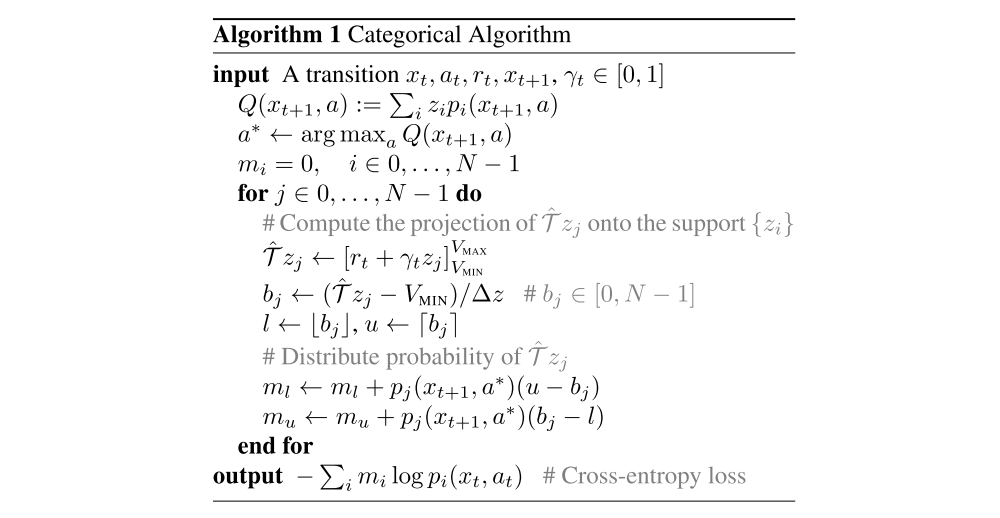
Assume we’ve just picked (xt, at, rt, xt+1) from the replay buffer in some variant of the DQN algorithm, so x is used to indicate states. The z0,…,zN−1 are the fixed global positions of the atoms. Let’s assume there’s just a global γ.
Let’s go through the algorithm in detail assuming we’re using a neural network for Z:
-
We feed xt+1 to our net which outputs an |A|×N matrix M(xt+1), i.e. each row corresponds to a single action and contains the probabilities for the N atoms. That is, the row for action a contains the vector

-
We compute all the
as follows:
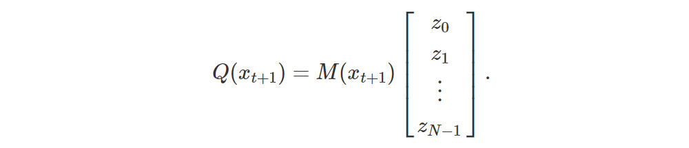
Note that Q(xt+1) is a column vector of length |A|.
-
Now we can determine the optimum action

Let q = (q0,…,qN−1) be the row of M(xt+1) corresponding to a∗.
-
m0,…,mN−1 will accumulate the probabilities of the aligned atoms of the target distribution rt + γ Z(xt+1, a∗). We start by zeroing them.
-
The non-aligned atoms of the target distribution are at positions

We clip those positions so that they are in [VMIN, VMAX], i.e. [z0, zN−1].
-
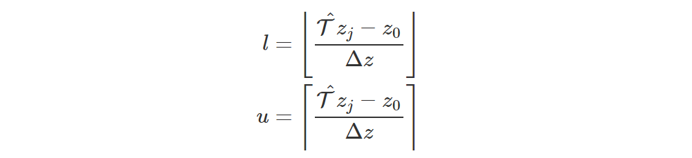
Assuming that the adjacent aligned atoms are at distance Δz, the indices of the closest aligned atoms on the left and on the right of T^zj are, respectively:
-
Now we need to split the weight of T^zj, which is qj, between ml and mr as we saw before. Note that
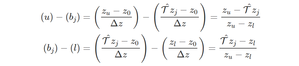
which means that, as we said before, the weight qj is split between zl and zu (indeed, u−bj+bj−l=1), and the contribution to ml is proportional to the distance of T^zj from zu. The more distant it is from zu, the higher the contribution to ml.
-
now we have the probabilities m0,…,mN−1 of the aligned atoms of rt + γ Z(xt+1, a∗) and, of course, the probabilities

of the aligned atoms of Z(xt, a), which are the ones we want to update. Thus
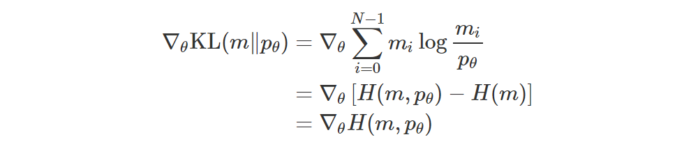
That is, we can just use the cross-entropy
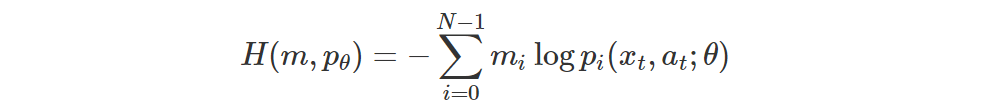
for the loss.