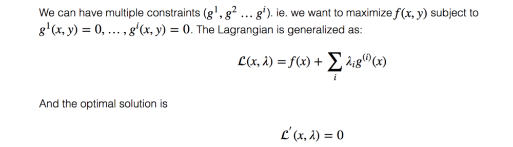
Concept 8: Dual Gradient Descent
Introduction
Dual Gradient Descent is a popular method for optimizing an objective under a constraint. In RL, it helps us to make better decisions.

The key idea is transforming the objective into a Lagrange dual function which can be optimized iteratively. The Lagrangian 𝓛 and the Lagrange dual function g is defined as:
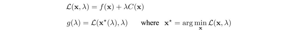
where λ is a scalar which we call the Lagrangian multiplier.
The dual function g is a lower bound for the original optimization problem. Indeed, if the function f is a convex function, the strong duality will often hold which say the maximum value of g equals the minimum values of the optimization problem. Hence, if we find λ that maximize g, we solve the optimization problem.
So we start with a random guess of λ and use any optimization method to solve this unconstrained objective.

Next, we will apply gradient ascent to update λ in order to maximize g. The gradient of g is:

i.e.

In step 1 below, we find the minimum x based on the current λ value, and then we take a gradient ascent step for g (step 2 and 3).
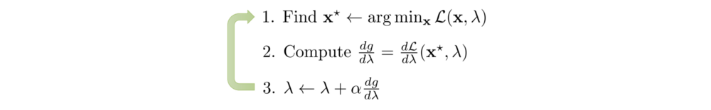
We alternate between minimizing the Lagrangian 𝓛 with respect to the primal variables x, and incrementing the Lagrange multiplier λ by its gradient. By repeating the iteration, the solution will converge.
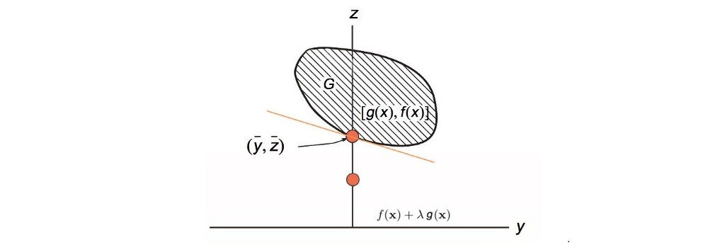
Visualization
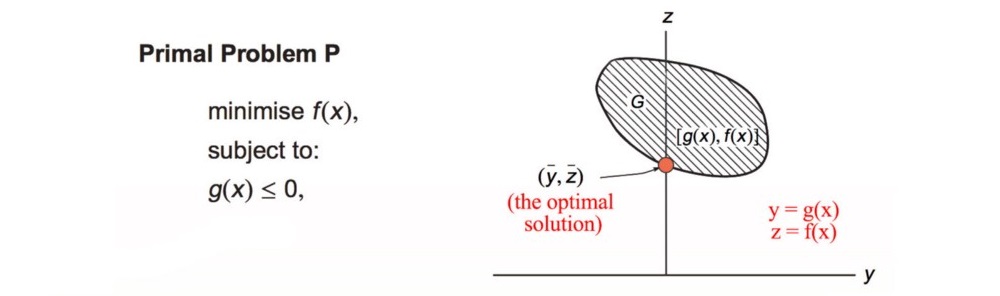
Let y = g(x) and z = f(x). y and z form a space G above and we plot z against y. Our solution is the orange dot above: the minimum f within the space G and g(x) = 0. The orange line below is our Lagrangian. Its slope equals λ and it touches the boundary of G.
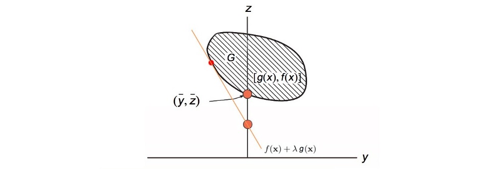
Then we use gradient ascent to adjust λ (the slope) for the maximum value f(x) that touches G with g(x) = 0.
Lagrange Multiplier
So what is this Lagrange multiplier? We can visualize f with a contour plot with different values of d. g is the constraint function.
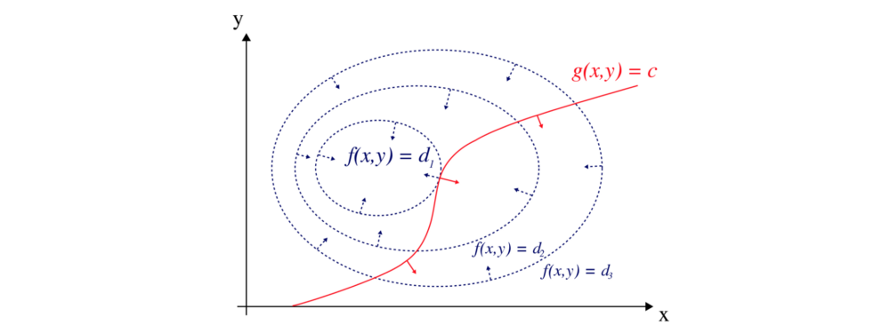
Geometrically, the optimal point lies where the gradient at f(x, y), the blue arrow, aligned with the gradient at g(x, y), the red arrow.
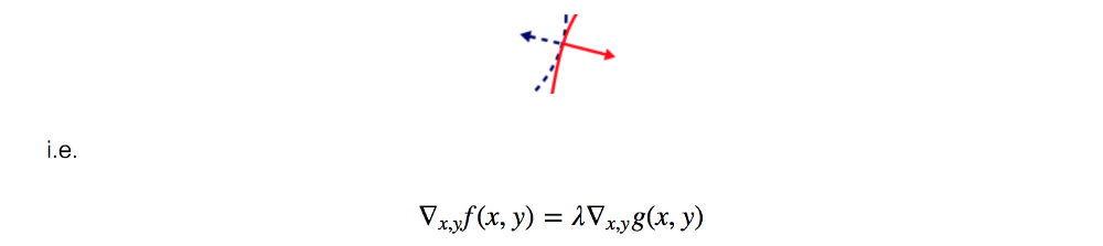
where λ is the Lagrange multiplier.